THE Analog Thing — Volume 5 — Worked examples & applications — THAT

Six fully-scaled patch walkthroughs with equations, SVG diagrams, and coefficient tables; companion to Vol 3 (elements) and Vol 6 (hybrid)

Introduction — How to Read This Volume

This volume presents six end-to-end worked demonstrations on THE ANALOG THING (THAT). Each demonstration follows the same structure: physical system and governing equations, machine scaling, element inventory, coefficient-potentiometer settings, patch description with an inline SVG signal-flow diagram, and expected oscilloscope output or phase portrait. The goal is to close the gap between a differential-equation description and a working patch that fits within THAT’s ±10 V machine unit.

Prerequisites. The reader should be comfortable with operational-amplifier integrators, the sign-inversion convention used by THAT’s integrators and summers, and the notion of machine time versus real time. Those topics are covered in Vol 3; the HYBRID port and digital host interaction appear in Vol 6.

Machine-unit reminder. THAT represents all quantities as voltages in the range ±10 V, which corresponds to the normalised machine unit ±1. Equations throughout this volume use machine-unit variables (dimensionless, bounded ±1) after scaling has been applied. Every integrator and summer on THAT inverts sign at its output; patch diagrams account for this by inserting explicit inverters where needed to maintain correct sign flow.

Element inventory — verified from First Steps v2 and Front schematic v1.3.

Block	Count	Notes
Integrators (INT1–INT5)	5	Each has 5 inputs (×1 ×1 ×1 ×10 ×10), one IC input, two output jacks
Summers (SUM1–SUM4)	4	Each has 7 inputs (×1 ×1 ×1 ×1 ×10 ×10 ×10), two output jacks
Inverters (INV1–INV4)	4	Unity gain, sign inversion
Multipliers (MUL1–MUL2)	2	Four-quadrant, output = +A·B (non-inverting; AD633-based)
Comparators (CMP1–CMP2)	2	Output selects ”>“-input when A+B > 0, else ”<“-input
Coefficient pots (PT1–PT8)	8	Range 0 to 1; connect input to ±1 for bipolar range via helper function
Machine units	—	Fixed ±1 jacks (±10 V) on panel

Note — THAT provides exactly 5 integrators, 4 summers, 4 inverters, 2 multipliers, and 2 comparators on a single board. Patches requiring more elements use the master/minion ribbon-cable chain (no limit on chain length per the First Steps manual).

THAT front panel perspective

Demo 1 — Simple Harmonic Oscillator (Undamped Pendulum)

Physical system and equations

The undamped simple pendulum (small-angle approximation, linearised) obeys:

θ̈ + ω₀² θ = 0

where θ is the angular displacement and ω₀ = √(g/L) is the natural frequency. Rearranging to isolate the highest derivative:

θ̈ = −ω₀² θ

Introducing the standard integrator chain:

θ̇  = ∫ θ̈ dt      (INT1)
θ   = ∫ θ̇  dt      (INT2)

Because each integrator inverts sign, INT1 accepts +ω₀²θ and produces −θ̇; INT2 accepts −θ̇ and produces +θ. The feedback path must then supply +ω₀²·(+θ) back to INT1’s input — no explicit inverter is needed because the two sign inversions cancel.

Scaling

Let the real pendulum have g = 9.81 m/s², L = 0.25 m, so ω₀ ≈ 6.26 rad/s and T ≈ 1.00 s.

For comfortable display on an oscilloscope, the machine period should be ≈ 1–2 s, so no time scaling is needed (real and machine time are equal, τ = 1).

Amplitude: set θ_max = 0.3 rad → normalise by 0.3 rad ⟹ machine variable X = θ/0.3. Peak machine value = 1.0 (full scale).

After scaling, the machine equation becomes:

Ẍ = −ω₀² X       with ω₀² ≈ 39.2  (machine time)

That coefficient (39.2) is far outside the range of a single pot (0–1). Use the ×10 weighted inputs on the integrators (gain 10) and set the pot to ω₀²/10 ≈ 0.39 — well within range.

Tip — When a coefficient exceeds 1.0, use the ×10 weighted input jack on the integrator or summer, then set the pot to the value divided by 10. Values above 10 require chaining two coefficients or a different time-scale factor.

Element inventory for this patch

Element	Role
INT1	Integrates −ω₀²X → produces −Ẋ
INT2	Integrates Ẋ (sign already correct) → produces +X
PT1	Set to 0.39 (= ω₀²/10), wired to ×10 input of INT1

Coefficient settings

Pot	Value	Connected to	Purpose
PT1	0.39	×10 input of INT1	Encodes ω₀² = 3.9 × 10
IC INT1	0.00	—	θ̇(0) = 0 (released from rest)
IC INT2	−1.00	−1 jack	θ(0) = +θ_max (IC sign inverts)

Patch SVG — Signal-flow diagram

<svg xmlns="http://www.w3.org/2000/svg" width="580" height="160" font-family="monospace" font-size="12">
  <!-- INT1 block -->
  <rect x="60" y="40" width="100" height="60" rx="6" fill="#d0e8ff" stroke="#336" stroke-width="1.5"/>
  <text x="110" y="65" text-anchor="middle" font-size="11" fill="#003">INT1</text>
  <text x="110" y="82" text-anchor="middle" font-size="10" fill="#003">∫ dt  (inv)</text>
  <!-- INT1 input arrow -->
  <line x1="20" y1="70" x2="60" y2="70" stroke="#333" stroke-width="1.5" marker-end="url(#arr)"/>
  <text x="36" y="63" text-anchor="middle" font-size="10">+ω₀²X</text>
  <!-- INT1 output arrow to INT2 -->
  <line x1="160" y1="70" x2="220" y2="70" stroke="#333" stroke-width="1.5" marker-end="url(#arr)"/>
  <text x="192" y="63" text-anchor="middle" font-size="10">−Ẋ</text>
  <!-- INT2 block -->
  <rect x="220" y="40" width="100" height="60" rx="6" fill="#d0e8ff" stroke="#336" stroke-width="1.5"/>
  <text x="270" y="65" text-anchor="middle" font-size="11" fill="#003">INT2</text>
  <text x="270" y="82" text-anchor="middle" font-size="10" fill="#003">∫ dt  (inv)</text>
  <!-- INT2 output -->
  <line x1="320" y1="70" x2="400" y2="70" stroke="#333" stroke-width="1.5" marker-end="url(#arr)"/>
  <text x="362" y="63" text-anchor="middle" font-size="10">+X (θ)</text>
  <!-- Feedback node -->
  <circle cx="420" cy="70" r="4" fill="#600"/>
  <!-- Feedback path down and back to INT1 input -->
  <polyline points="420,70 420,130 30,130 30,70" fill="none" stroke="#600" stroke-width="1.5" stroke-dasharray="6,3" marker-end="url(#arr)"/>
  <text x="225" y="148" text-anchor="middle" font-size="10" fill="#600">feedback: X → PT1(×10 in) → INT1</text>
  <!-- Output jack label -->
  <rect x="400" y="50" width="70" height="25" rx="4" fill="#fff8cc" stroke="#aa8800" stroke-width="1"/>
  <text x="435" y="67" text-anchor="middle" font-size="10">X-jack / Y-jack</text>
  <!-- PT1 label -->
  <rect x="20" y="10" width="60" height="20" rx="3" fill="#eee" stroke="#888"/>
  <text x="50" y="24" text-anchor="middle" font-size="10">PT1 = 0.39</text>
  <line x1="50" y1="30" x2="50" y2="70" stroke="#888" stroke-width="1" stroke-dasharray="3,2"/>
  <!-- arrowhead marker -->
  <defs>
    <marker id="arr" markerWidth="8" markerHeight="8" refX="6" refY="3" orient="auto">
      <path d="M0,0 L0,6 L8,3 z" fill="#333"/>
    </marker>
  </defs>
</svg>

Expected output

With mode selector in REP and OP-time set to ≈ 2 s, the oscilloscope (X vs time) displays a clean sinusoid at ≈ 1 Hz. In X-Y mode (X = θ, Y = Ẋ) the phase portrait is a closed ellipse — the hallmark of a conservative oscillator. Changing PT1 shifts the frequency; adjusting the IC jack of INT2 changes amplitude.

Demo 2 — Damped Pendulum (Mass-Spring-Damper)

Physical system and equations

The First Steps manual (Section 9.2) presents the mass-spring-damper as a direct companion to the simple oscillator. Adding a velocity-proportional damping term d gives:

θ̈ + d·θ̇ + ω₀² θ = 0

Rearranging:

θ̈ = −d·θ̇ − ω₀² θ

Scaling

Using the same parameter set as Demo 1 (ω₀² ≈ 39.2, handled by ×10 input + pot ≈ 0.39) and adding a damping coefficient d = 2·ζ·ω₀ where ζ is the damping ratio. For ζ = 0.3 (underdamped, visible decay):

d = 2 × 0.3 × 6.26 ≈ 3.76

d = 3.76 is handled by a ×10 weighted input with pot set to 0.376.

Element inventory

Element	Role
INT1	Integrates (−d·Ẋ − ω₀²·X) → −Ẋ
INT2	Integrates Ẋ → +X
PT1	0.39, ×10 input of INT1 — encodes ω₀²
PT2	0.376, ×10 input of INT1 — encodes d (feedback from −Ẋ)

Coefficient settings

Pot	Value	Connected to	Purpose
PT1	0.39	×10 input INT1	ω₀² term from X feedback
PT2	0.376	×10 input INT1	damping d from −Ẋ (INT1 output)
IC INT1	0.00	—	Ẋ(0) = 0
IC INT2	−1.00	−1 jack	X(0) = +1 (maximum displacement)

Note — The output of INT1 is −Ẋ. Feeding −Ẋ back into INT1’s ×10 input (which will invert again to +Ẋ inside the integrator) implements the +d·Ẋ restoring term correctly. No separate inverter is needed for the damping path.

Patch SVG

<svg xmlns="http://www.w3.org/2000/svg" width="640" height="200" font-family="monospace" font-size="12">
  <defs>
    <marker id="arr2" markerWidth="8" markerHeight="8" refX="6" refY="3" orient="auto">
      <path d="M0,0 L0,6 L8,3 z" fill="#333"/>
    </marker>
  </defs>
  <!-- INT1 -->
  <rect x="80" y="60" width="110" height="70" rx="6" fill="#d0e8ff" stroke="#336" stroke-width="1.5"/>
  <text x="135" y="88" text-anchor="middle" font-size="11" fill="#003">INT1</text>
  <text x="135" y="105" text-anchor="middle" font-size="10" fill="#003">−d·Ẋ−ω₀²X→−Ẋ</text>
  <!-- INT2 -->
  <rect x="280" y="60" width="110" height="70" rx="6" fill="#d0e8ff" stroke="#336" stroke-width="1.5"/>
  <text x="335" y="88" text-anchor="middle" font-size="11" fill="#003">INT2</text>
  <text x="335" y="105" text-anchor="middle" font-size="10" fill="#003">−Ẋ → +X</text>
  <!-- INT1 to INT2 -->
  <line x1="190" y1="95" x2="280" y2="95" stroke="#333" stroke-width="1.5" marker-end="url(#arr2)"/>
  <text x="235" y="88" text-anchor="middle" font-size="10">−Ẋ</text>
  <!-- INT2 output node -->
  <circle cx="430" cy="95" r="4" fill="#600"/>
  <line x1="390" y1="95" x2="450" y2="95" stroke="#333" stroke-width="1.5" marker-end="url(#arr2)"/>
  <text x="418" y="88" text-anchor="middle" font-size="10">+X</text>
  <!-- output label -->
  <rect x="450" y="78" width="80" height="22" rx="4" fill="#fff8cc" stroke="#aa8800"/>
  <text x="490" y="93" text-anchor="middle" font-size="10">X-out (θ)</text>
  <!-- X feedback path (ω₀²) -->
  <polyline points="430,95 430,170 40,170 40,75 80,75"
    fill="none" stroke="#600" stroke-width="1.5" stroke-dasharray="6,3" marker-end="url(#arr2)"/>
  <text x="240" y="185" text-anchor="middle" font-size="10" fill="#600">X → PT1(×10) → INT1 input (ω₀² path)</text>
  <!-- −Ẋ feedback (damping) -->
  <polyline points="190,95 220,95 220,150 55,150 55,88 80,88"
    fill="none" stroke="#a00" stroke-width="1.5" stroke-dasharray="4,2" marker-end="url(#arr2)"/>
  <text x="135" y="143" text-anchor="middle" font-size="10" fill="#a00">−Ẋ → PT2(×10) → INT1 input (damping path)</text>
  <!-- PT labels -->
  <rect x="5" y="30" width="60" height="18" rx="3" fill="#eee" stroke="#888"/>
  <text x="35" y="43" text-anchor="middle" font-size="10">PT1=0.39</text>
  <rect x="75" y="10" width="65" height="18" rx="3" fill="#eee" stroke="#888"/>
  <text x="107" y="23" text-anchor="middle" font-size="10">PT2=0.376</text>
</svg>

Expected output and phase portrait

The oscilloscope (X vs time) shows exponentially decaying sinusoidal oscillation. In X-Y mode (X = θ, Y = Ẋ = −INT1 output), the phase portrait is an inward spiral converging on the origin. Increasing PT2 tightens the spiral (heavier damping); at PT2 ≈ 0.63 (ζ = 1, critically damped) the spiral becomes a direct approach to the origin with no overshoot.

ζ (damping ratio)	PT2 value	Phase-portrait character
0.1 (lightly damped)	0.125	Wide, slowly decaying spiral
0.3 (typical)	0.376	Moderate spiral, ~3 cycles to rest
1.0 (critical)	1.254 (use ×10 + pot 0.125)	Direct approach, no overshoot
> 1.0 (overdamped)	higher	No oscillation, pure exponential

Demo 3 — Lorenz Attractor

Physical system and equations

The Lorenz system (1963) is the canonical chaotic attractor, derived from a simplified model of atmospheric convection. Its three-dimensional state evolves as:

ẋ = σ(y − x)
ẏ = x(ρ − z) − y
ż = xy − βz

Classic parameter values: σ = 10, ρ = 28, β = 8/3 ≈ 2.667. The attractor wings span roughly x ∈ [−20, +20], y ∈ [−28, +28], z ∈ [0, 50].

This is one of the nine demonstrations in the First Steps manual (Section 9.7). It requires all five integrators, both multipliers, multiple summers, and all eight coefficient potentiometers on a single THAT — the most element-intensive patch in the manual.

Scaling

Raw variable ranges must map into ±1 machine units. Choose normalisation constants:

X = x/20    (x ∈ [−20,+20] → X ∈ [−1,+1])
Y = y/30    (y ∈ [−30,+30] → Y ∈ [−1,+1])
Z = z/50    (z ∈  [0,+50]  → Z ∈  [0,+1])

After substitution (writing lowercase for real, uppercase for machine):

Ẋ = σ(Y·30/20 − X)           = σ(1.5Y − X)
Ẏ = (20X)(ρ − 50Z)/30 − Y    = (20X·ρ − 1000X·Z)/30 − Y
Ż = (20X)(30Y)/50 − βZ       = 12XY − βZ

Insert machine time τ (real time t = τ/k, where k is the time-scale factor). Choosing k = 0.1 compresses real dynamics by 10× so that one revolution of the attractor takes ≈ 0.5–2 s on the oscilloscope:

dX/dτ = 0.1·σ(1.5Y − X)          = 1.5Y − X       (σ=10, absorbs into pot)
dY/dτ = 0.1(20X·ρ/30 − Y) − 0.1·(1000/30)·XZ
dZ/dτ = 0.1(12XY − βZ)

Note — Exact coefficient values for the scaled Lorenz system depend on the chosen normalisation and time constant. The First Steps manual presents this patch qualitatively; the operator is expected to tune PT1–PT8 empirically to observe the attractor. The values below represent one widely used starting point. Overload will occur if scaling constants are too small.

Element inventory

Element	Role
INT1	Integrates dX/dτ → X
INT2	Integrates dY/dτ → Y
INT3	Integrates dZ/dτ → Z
MUL1	Computes X·Z (needed for Y equation)
MUL2	Computes X·Y (needed for Z equation)
SUM1	Forms −dX/dτ from σ(Y−X)
SUM2	Forms −dY/dτ
SUM3	Forms −dZ/dτ
INV1, INV2	Sign correction where needed
PT1–PT8	Encodes σ, ρ, β, and scale terms

Coefficient settings (starting point)

Pot	Approx. value	Term encoded
PT1	0.10	σ/10 × x-path gain (×10 input)
PT2	0.15	σ·1.5/10 — Y path into ẋ (×10 input)
PT3	0.28	ρ/100 — x·ρ term (via MUL1 × PT, ×10 input)
PT4	0.10	Scale on X·Z → Y̊
PT5	0.10	Y damping in Ẏ
PT6	0.12	X·Y → Ż gain
PT7	0.027	β/10 — Z damping
PT8	(spare or IC)	IC offset for Z if needed

Tip — Start with all pots at 0, then increase PT1 and PT2 first (they drive the x-loop). Once X oscillates, bring in PT3 and PT4 to couple Y, then PT6 and PT7 for Z. The attractor will snap into its characteristic butterfly shape once all three loops are active and within scale.

Patch SVG — Three-loop signal flow

<svg xmlns="http://www.w3.org/2000/svg" width="700" height="320" font-family="monospace" font-size="11">
  <defs>
    <marker id="arL" markerWidth="8" markerHeight="8" refX="6" refY="3" orient="auto">
      <path d="M0,0 L0,6 L8,3 z" fill="#333"/>
    </marker>
  </defs>
  <!-- ===== X loop ===== -->
  <rect x="30" y="20" width="90" height="50" rx="5" fill="#cce8cc" stroke="#336"/>
  <text x="75" y="42" text-anchor="middle" font-size="10">SUM1</text>
  <text x="75" y="56" text-anchor="middle" font-size="9">σ(Y−X)</text>
  <line x1="120" y1="45" x2="160" y2="45" stroke="#333" stroke-width="1.5" marker-end="url(#arL)"/>
  <rect x="160" y="20" width="80" height="50" rx="5" fill="#d0e8ff" stroke="#336"/>
  <text x="200" y="42" text-anchor="middle" font-size="10">INT1</text>
  <text x="200" y="56" text-anchor="middle" font-size="9">→ X</text>
  <!-- X output and feedback -->
  <circle cx="290" cy="45" r="4" fill="#600"/>
  <line x1="240" y1="45" x2="320" y2="45" stroke="#333" stroke-width="1.5" marker-end="url(#arL)"/>
  <text x="282" y="38" font-size="9">X</text>
  <polyline points="290,45 290,100 75,100 75,70" fill="none" stroke="#600" stroke-width="1.2" stroke-dasharray="5,3" marker-end="url(#arL)"/>

  <!-- ===== Y loop ===== -->
  <rect x="30" y="130" width="90" height="50" rx="5" fill="#cce8cc" stroke="#336"/>
  <text x="75" y="152" text-anchor="middle" font-size="10">SUM2</text>
  <text x="75" y="166" text-anchor="middle" font-size="9">x(ρ−z)−y</text>
  <line x1="120" y1="155" x2="160" y2="155" stroke="#333" stroke-width="1.5" marker-end="url(#arL)"/>
  <rect x="160" y="130" width="80" height="50" rx="5" fill="#d0e8ff" stroke="#336"/>
  <text x="200" y="152" text-anchor="middle" font-size="10">INT2</text>
  <text x="200" y="166" text-anchor="middle" font-size="9">→ Y</text>
  <circle cx="290" cy="155" r="4" fill="#600"/>
  <line x1="240" y1="155" x2="320" y2="155" stroke="#333" stroke-width="1.5" marker-end="url(#arL)"/>
  <text x="282" y="148" font-size="9">Y</text>
  <polyline points="290,155 290,210 75,210 75,180" fill="none" stroke="#600" stroke-width="1.2" stroke-dasharray="5,3" marker-end="url(#arL)"/>

  <!-- ===== Z loop ===== -->
  <rect x="30" y="240" width="90" height="50" rx="5" fill="#cce8cc" stroke="#336"/>
  <text x="75" y="262" text-anchor="middle" font-size="10">SUM3</text>
  <text x="75" y="276" text-anchor="middle" font-size="9">xy−βz</text>
  <line x1="120" y1="265" x2="160" y2="265" stroke="#333" stroke-width="1.5" marker-end="url(#arL)"/>
  <rect x="160" y="240" width="80" height="50" rx="5" fill="#d0e8ff" stroke="#336"/>
  <text x="200" y="262" text-anchor="middle" font-size="10">INT3</text>
  <text x="200" y="276" text-anchor="middle" font-size="9">→ Z</text>
  <circle cx="290" cy="265" r="4" fill="#600"/>
  <line x1="240" y1="265" x2="320" y2="265" stroke="#333" stroke-width="1.5" marker-end="url(#arL)"/>
  <text x="282" y="258" font-size="9">Z</text>
  <polyline points="290,265 290,308 75,308 75,290" fill="none" stroke="#600" stroke-width="1.2" stroke-dasharray="5,3" marker-end="url(#arL)"/>

  <!-- ===== Multipliers ===== -->
  <rect x="340" y="90" width="80" height="45" rx="5" fill="#ffe0c0" stroke="#a63"/>
  <text x="380" y="110" text-anchor="middle" font-size="10">MUL1</text>
  <text x="380" y="125" text-anchor="middle" font-size="9">X·Z</text>
  <rect x="340" y="190" width="80" height="45" rx="5" fill="#ffe0c0" stroke="#a63"/>
  <text x="380" y="210" text-anchor="middle" font-size="10">MUL2</text>
  <text x="380" y="225" text-anchor="middle" font-size="9">X·Y</text>

  <!-- X,Z → MUL1 -->
  <line x1="320" y1="45" x2="350" y2="105" stroke="#888" stroke-width="1" stroke-dasharray="3,2" marker-end="url(#arL)"/>
  <line x1="320" y1="265" x2="350" y2="125" stroke="#888" stroke-width="1" stroke-dasharray="3,2" marker-end="url(#arL)"/>
  <!-- MUL1 → SUM2 -->
  <line x1="420" y1="112" x2="450" y2="112" stroke="#a63" stroke-width="1.2" marker-end="url(#arL)"/>
  <polyline points="450,112 450,155 120,155" fill="none" stroke="#a63" stroke-width="1.2" marker-end="url(#arL)"/>

  <!-- X,Y → MUL2 -->
  <line x1="320" y1="45" x2="350" y2="200" stroke="#888" stroke-width="1" stroke-dasharray="3,2"/>
  <line x1="320" y1="155" x2="350" y2="215" stroke="#888" stroke-width="1" stroke-dasharray="3,2"/>
  <!-- MUL2 → SUM3 -->
  <line x1="420" y1="212" x2="460" y2="212" stroke="#a63" stroke-width="1.2" marker-end="url(#arL)"/>
  <polyline points="460,212 460,265 120,265" fill="none" stroke="#a63" stroke-width="1.2" marker-end="url(#arL)"/>

  <!-- Output labels -->
  <rect x="325" y="35" width="55" height="18" rx="3" fill="#fff8cc" stroke="#aa8800"/>
  <text x="352" y="48" text-anchor="middle" font-size="9">X → x-jack</text>
  <rect x="325" y="145" width="55" height="18" rx="3" fill="#fff8cc" stroke="#aa8800"/>
  <text x="352" y="158" text-anchor="middle" font-size="9">Y → y-jack</text>
</svg>

Expected output

Set the oscilloscope to X-Y mode with X-jack → horizontal, Y-jack → vertical. After a transient of a few seconds, the display settles onto the characteristic butterfly-shaped Lorenz attractor — two lobes that the trajectory orbits chaotically, never repeating. In REP mode (cycle period ≈ 5–10 s), each sweep traces a slightly different path, demonstrating sensitive dependence on initial conditions. The Z channel, connected to the U-jack and routed to the panel meter, shows aperiodic excursions between approximately 0.1 and 0.9 (machine units).

Note — The Lorenz attractor is chaotic; identical initial conditions in hardware are not achievable to infinite precision. Each REP cycle will trace a unique, non-repeating orbit — this is the intended and correct behaviour, not a fault.

Demo 4 — Van der Pol Oscillator

Physical system and equations

The Van der Pol oscillator is a nonlinear relaxation oscillator that exhibits a stable limit cycle. It arises in vacuum-tube circuits, cardiac pacemaker models, and neuronal dynamics. The governing equation is:

ẍ − μ(1 − x²)ẋ + x = 0

where μ > 0 is the nonlinearity parameter. For μ ≪ 1 the oscillator is nearly sinusoidal; for μ ≫ 1 it becomes a relaxation oscillator with sharp transitions.

Rearranging:

ẍ = μ(1 − x²)ẋ − x

The term (1 − x²)ẋ requires forming x², which needs a multiplier, and then multiplying x² by ẋ, which needs a second multiplier. A single THAT (2 multipliers) is sufficient for this patch.

Scaling

Choose μ = 1 (smooth limit cycle, period ≈ 6.6 s real time). With machine time τ = t (no scaling), x_max ≈ 2. Normalise: X = x/2.

Substituting X = x/2 → x = 2X, ẋ = 2Ẋ:

2Ẍ = μ(1 − 4X²)·2Ẋ − 2X
Ẍ  = μ(1 − 4X²)Ẋ − X

With μ = 1:

Ẍ = Ẋ − 4X²Ẋ − X

The term Ẋ enters INT1 directly (pot = 1.0 — but this exceeds pot range; use ×1 input or reduce μ).
The term −4X²Ẋ requires MUL1 (compute X·X = X²), then MUL2 (compute X²·Ẋ), then scale by −4 → use ×10 input with pot = 0.4.
The term −X enters INT1 from the X feedback (pot = 1.0 at ×1 input).

Tip — Choosing μ = 0.5 and leaving x unnormalised (x_max ≈ 2, pot ×1 with value 0.5 for the μ·Ẋ term) is a cleaner starting point. Tune μ from near zero upward; the limit cycle appears above μ ≈ 0.1.

Element inventory

Element	Role
INT1	Integrates ẍ → Ẋ
INT2	Integrates Ẋ → X
MUL1	Forms +X·X = +X² (output = +X²; non-inverting)
MUL2	Forms +X²·Ẋ (output = +X²·Ẋ; non-inverting; negate via inverter as needed)
SUM1	Sums contributions to ẍ
INV1	Corrects sign as needed
PT1	μ (linear positive-damping term)
PT2	4μ (nonlinear negative-damping coefficient)
PT3	1.0 (spring restoring term, or use ×1 input directly)

Coefficient settings (μ = 1, normalised X = x/2)

Pot	Value	Connected to
PT1	1.00	×1 input of SUM1 — Ẋ gain (μ term)
PT2	0.40	×10 input of SUM1 — 4X²Ẋ gain
PT3	1.00	×1 input of SUM1 — X feedback (spring)
IC INT1	0.00	Ẋ(0) = 0
IC INT2	−0.50	X(0) = +0.5 (small perturbation from origin)

Patch SVG — Limit-cycle topology

<svg xmlns="http://www.w3.org/2000/svg" width="680" height="260" font-family="monospace" font-size="11">
  <defs>
    <marker id="arVP" markerWidth="8" markerHeight="8" refX="6" refY="3" orient="auto">
      <path d="M0,0 L0,6 L8,3 z" fill="#333"/>
    </marker>
  </defs>
  <!-- SUM1 -->
  <rect x="20" y="80" width="90" height="60" rx="5" fill="#cce8cc" stroke="#336"/>
  <text x="65" y="106" text-anchor="middle" font-size="10">SUM1</text>
  <text x="65" y="120" text-anchor="middle" font-size="9">Ẋ−4X²Ẋ−X</text>
  <!-- INT1 -->
  <rect x="150" y="80" width="90" height="60" rx="5" fill="#d0e8ff" stroke="#336"/>
  <text x="195" y="106" text-anchor="middle" font-size="10">INT1</text>
  <text x="195" y="120" text-anchor="middle" font-size="9">ẍ → Ẋ</text>
  <!-- INT2 -->
  <rect x="300" y="80" width="90" height="60" rx="5" fill="#d0e8ff" stroke="#336"/>
  <text x="345" y="106" text-anchor="middle" font-size="10">INT2</text>
  <text x="345" y="120" text-anchor="middle" font-size="9">Ẋ → X</text>
  <!-- MUL1 -->
  <rect x="430" y="30" width="80" height="45" rx="5" fill="#ffe0c0" stroke="#a63"/>
  <text x="470" y="50" text-anchor="middle" font-size="10">MUL1</text>
  <text x="470" y="65" text-anchor="middle" font-size="9">+X·X=+X²</text>
  <!-- MUL2 -->
  <rect x="430" y="165" width="80" height="45" rx="5" fill="#ffe0c0" stroke="#a63"/>
  <text x="470" y="185" text-anchor="middle" font-size="10">MUL2</text>
  <text x="470" y="200" text-anchor="middle" font-size="9">X²·Ẋ</text>
  <!-- Arrows SUM1→INT1→INT2 -->
  <line x1="110" y1="110" x2="150" y2="110" stroke="#333" stroke-width="1.5" marker-end="url(#arVP)"/>
  <line x1="240" y1="110" x2="300" y2="110" stroke="#333" stroke-width="1.5" marker-end="url(#arVP)"/>
  <!-- INT1 output node (Ẋ) -->
  <circle cx="260" cy="110" r="4" fill="#009"/>
  <text x="261" y="103" font-size="9" fill="#009">Ẋ</text>
  <!-- INT2 output node (X) -->
  <circle cx="430" cy="110" r="4" fill="#600"/>
  <line x1="390" y1="110" x2="460" y2="110" stroke="#333" stroke-width="1.5" marker-end="url(#arVP)"/>
  <text x="413" y="103" font-size="9">X</text>
  <!-- X → MUL1 (both inputs) -->
  <line x1="430" y1="110" x2="480" y2="85" stroke="#600" stroke-width="1.2" stroke-dasharray="4,2" marker-end="url(#arVP)"/>
  <line x1="430" y1="110" x2="480" y2="72" stroke="#600" stroke-width="1.2" stroke-dasharray="4,2"/>
  <!-- −X² from MUL1 → MUL2 input -->
  <line x1="430" y1="52" x2="410" y2="52" stroke="#a63" stroke-width="1.2" marker-end="url(#arVP)"/>
  <polyline points="410,52 410,185 430,185" fill="none" stroke="#a63" stroke-width="1.2" marker-end="url(#arVP)"/>
  <!-- Ẋ → MUL2 input -->
  <line x1="260" y1="110" x2="260" y2="212" stroke="#009" stroke-width="1.2" stroke-dasharray="4,2" marker-end="url(#arVP)"/>
  <line x1="260" y1="212" x2="430" y2="212" stroke="#009" stroke-width="1.2" stroke-dasharray="4,2" marker-end="url(#arVP)"/>
  <!-- MUL2 → SUM1 (nonlinear damping) -->
  <polyline points="430,187 380,187 380,240 65,240 65,140" fill="none" stroke="#a63" stroke-width="1.2" stroke-dasharray="5,3" marker-end="url(#arVP)"/>
  <text x="220" y="255" font-size="9" fill="#a63">−4X²Ẋ feedback (PT2×10)</text>
  <!-- X → SUM1 (spring term) -->
  <polyline points="430,110 430,130 570,130 570,260 10,260 10,110 20,110" fill="none" stroke="#600" stroke-width="1.2" stroke-dasharray="6,3" marker-end="url(#arVP)"/>
  <text x="290" y="15" font-size="9" fill="#600">X spring feedback (PT3)</text>
  <!-- Ẋ → SUM1 (linear damping) -->
  <polyline points="260,110 260,72 10,72 10,100 20,100" fill="none" stroke="#009" stroke-width="1.2" stroke-dasharray="6,3" marker-end="url(#arVP)"/>
  <text x="135" y="65" font-size="9" fill="#009">Ẋ linear term (PT1)</text>
  <!-- Output labels -->
  <rect x="460" y="100" width="65" height="18" rx="3" fill="#fff8cc" stroke="#aa8800"/>
  <text x="492" y="113" text-anchor="middle" font-size="9">X → x-jack</text>
</svg>

Expected output

With μ near zero, the phase portrait is a nearly circular closed loop (near-sinusoidal). As μ increases toward 1, the loop distorts into a rounded rectangle. At μ ≫ 1 (set PT1 near 1, ×10 input → effectively μ = 10), the portrait becomes a relaxation-oscillator sawtooth: rapid slewing on the horizontal sides, slow drift on the vertical sides. The limit cycle is stable — perturbations from any initial condition converge onto the same closed orbit.

Demo 5 — Predator-Prey Dynamics (Lotka-Volterra)

Physical system and equations

The Lotka-Volterra equations model the interaction between a prey population R (rabbits) and a predator population F (foxes):

Ṙ =  α·R − β·R·F        (prey grows, is hunted)
Ḟ = −γ·F + δ·R·F        (predators die, fed by hunting)

Classic parameters: α = 0.67, β = 1.33, γ = 1.00, δ = 1.00.

The system is conservative (no damping); trajectories in the (R, F) plane are closed orbits around the non-trivial equilibrium (R*, F*) = (γ/δ, α/β) = (1.0, 0.50).

This corresponds to the First Steps manual Section 9.6 (“Hunter and Prey Population Dynamics”).

Scaling

Natural variables R and F range from roughly 0 to 2 in normalised units. Scale:

X = R/2    Y = F/2

Machine equations:

Ẋ =  α·X − 2β·X·Y     =  0.67X − 2.66·X·Y
Ẏ = −γ·Y + 2δ·X·Y     = −1.00·Y + 2.00·X·Y

The term X·Y requires one multiplier (MUL1). The second multiplier is free for other purposes or can double the X·Y product with a pot.

Note — The Lotka-Volterra system requires only one multiplier because both coupling terms share the same X·Y product. MUL1 forms X·Y; two separate pots scale it to 2.66 and 2.00 for the two equations respectively.

Element inventory

Element	Role
INT1	Integrates Ẋ → X (prey population)
INT2	Integrates Ẏ → Y (predator population)
MUL1	Forms +X·Y (four-quadrant, non-inverting); output routed via inverter for negated coupling
SUM1	Computes −Ẋ from α·X and 2β·X·Y
SUM2	Computes −Ẏ from γ·Y and 2δ·X·Y
PT1	α = 0.67
PT2	2β = 0.266 (×10 input → effective 2.66)
PT3	γ = 1.00
PT4	2δ = 0.20 (×10 input → effective 2.00)

Coefficient settings

Pot	Value	Connected to	Purpose
PT1	0.67	×1 input SUM1	α — prey growth rate
PT2	0.266	×10 input SUM1	2β — predation rate (from X·Y via inverter)
PT3	1.00	×1 input SUM2	γ — predator death rate (from Y)
PT4	0.20	×10 input SUM2	2δ — predator growth (from X·Y)
IC INT1	−0.75	−1 jack scaled	X(0) = 0.75 (75% of max prey)
IC INT2	−0.25	pot at 0.25 from −1	Y(0) = 0.25 (25% of max predator)

Patch SVG

<svg xmlns="http://www.w3.org/2000/svg" width="640" height="240" font-family="monospace" font-size="11">
  <defs>
    <marker id="arLV" markerWidth="8" markerHeight="8" refX="6" refY="3" orient="auto">
      <path d="M0,0 L0,6 L8,3 z" fill="#333"/>
    </marker>
  </defs>
  <!-- SUM1 -->
  <rect x="20" y="30" width="90" height="55" rx="5" fill="#cce8cc" stroke="#336"/>
  <text x="65" y="53" text-anchor="middle" font-size="10">SUM1</text>
  <text x="65" y="67" text-anchor="middle" font-size="9">αX−2βXY</text>
  <!-- INT1 -->
  <rect x="160" y="30" width="90" height="55" rx="5" fill="#d0e8ff" stroke="#336"/>
  <text x="205" y="53" text-anchor="middle" font-size="10">INT1</text>
  <text x="205" y="67" text-anchor="middle" font-size="9">→ X (prey)</text>
  <line x1="110" y1="57" x2="160" y2="57" stroke="#333" stroke-width="1.5" marker-end="url(#arLV)"/>
  <!-- SUM2 -->
  <rect x="20" y="150" width="90" height="55" rx="5" fill="#cce8cc" stroke="#336"/>
  <text x="65" y="173" text-anchor="middle" font-size="10">SUM2</text>
  <text x="65" y="187" text-anchor="middle" font-size="9">−γY+2δXY</text>
  <!-- INT2 -->
  <rect x="160" y="150" width="90" height="55" rx="5" fill="#d0e8ff" stroke="#336"/>
  <text x="205" y="173" text-anchor="middle" font-size="10">INT2</text>
  <text x="205" y="187" text-anchor="middle" font-size="9">→ Y (pred.)</text>
  <line x1="110" y1="177" x2="160" y2="177" stroke="#333" stroke-width="1.5" marker-end="url(#arLV)"/>
  <!-- MUL1 -->
  <rect x="360" y="90" width="80" height="45" rx="5" fill="#ffe0c0" stroke="#a63"/>
  <text x="400" y="110" text-anchor="middle" font-size="10">MUL1</text>
  <text x="400" y="125" text-anchor="middle" font-size="9">+X·Y</text>
  <!-- X output node -->
  <circle cx="310" cy="57" r="4" fill="#006600"/>
  <line x1="250" y1="57" x2="340" y2="57" stroke="#333" stroke-width="1.5" marker-end="url(#arLV)"/>
  <text x="285" y="50" font-size="9" fill="#006600">X</text>
  <!-- Y output node -->
  <circle cx="310" cy="177" r="4" fill="#660000"/>
  <line x1="250" y1="177" x2="340" y2="177" stroke="#333" stroke-width="1.5" marker-end="url(#arLV)"/>
  <text x="285" y="170" font-size="9" fill="#660000">Y</text>
  <!-- X,Y → MUL1 -->
  <line x1="310" y1="57" x2="370" y2="100" stroke="#006600" stroke-width="1.2" stroke-dasharray="4,2" marker-end="url(#arLV)"/>
  <line x1="310" y1="177" x2="370" y2="130" stroke="#660000" stroke-width="1.2" stroke-dasharray="4,2" marker-end="url(#arLV)"/>
  <!-- MUL1 → SUM1 (predation on prey) -->
  <polyline points="360,112 320,112 320,20 65,20 65,30"
    fill="none" stroke="#a63" stroke-width="1.2" stroke-dasharray="5,3" marker-end="url(#arLV)"/>
  <text x="190" y="13" font-size="9" fill="#a63">XY → PT2(×10) → SUM1 (−predation)</text>
  <!-- MUL1 → SUM2 (predator growth) -->
  <polyline points="360,120 330,120 330,220 65,220 65,205"
    fill="none" stroke="#a63" stroke-width="1.2" stroke-dasharray="5,3" marker-end="url(#arLV)"/>
  <text x="190" y="233" font-size="9" fill="#a63">XY → PT4(×10) → SUM2 (+predator growth)</text>
  <!-- X feedback → SUM1 (growth) -->
  <polyline points="310,57 540,57 540,10 65,10" fill="none" stroke="#006600" stroke-width="1.2" stroke-dasharray="6,3" marker-end="url(#arLV)"/>
  <!-- Y feedback → SUM2 (death) -->
  <polyline points="310,177 550,177 550,230 65,230" fill="none" stroke="#660000" stroke-width="1.2" stroke-dasharray="6,3" marker-end="url(#arLV)"/>
  <!-- Output labels -->
  <rect x="330" y="45" width="65" height="18" rx="3" fill="#fff8cc" stroke="#aa8800"/>
  <text x="362" y="58" text-anchor="middle" font-size="9">X → x-jack</text>
  <rect x="330" y="165" width="65" height="18" rx="3" fill="#fff8cc" stroke="#aa8800"/>
  <text x="362" y="178" text-anchor="middle" font-size="9">Y → y-jack</text>
</svg>

Expected output

Run in REP mode with OP-time set to 5–10 s. On the oscilloscope in X-Y mode, the phase portrait shows a closed oval orbit — prey on the horizontal axis, predator on the vertical. The orbit is traversed counter-clockwise: prey peaks first, predator peaks follow with a quarter-period lag.

In time-domain mode, X and Y appear as periodic oscillations with predator lagging prey. The period can be estimated analytically as T ≈ 2π/√(α·γ) ≈ 2π/0.82 ≈ 7.7 s (real time); adjust by changing PT1 and PT3.

Note — The Lotka-Volterra system is structurally neutral — each initial condition produces a different closed orbit. There is no global attractor. Introducing a small saturation term (1 − R/K type) converts the neutrally stable cycles into a stable limit cycle, but requires a multiplier and additional patching.

Demo 6 — Euler Spiral (Cornu Spiral / Clothoid)

Physical system and equations

The Euler spiral (also called the Cornu spiral or clothoid) is defined by the parametric equations:

x(t) = ∫₀ᵗ cos(πs²/2) ds
y(t) = ∫₀ᵗ sin(πs²/2) ds

The curvature increases linearly with arc length, making this curve essential in road and railway transition-curve design (see Vol 3 for mathematical background). Differentiating:

ẋ = cos(πt²/2)
ẏ = sin(πt²/2)

Both ẋ and ẏ are the real and imaginary parts of exp(iπt²/2). On an analog computer, the sine and cosine can be generated by a coupled-oscillator circuit whose frequency increases linearly with time. Differentiating again:

ẍ = −πt·sin(πt²/2) = −πt·ẏ
ÿ  =  πt·cos(πt²/2) =  πt·ẋ

The factor πt increases linearly — it is itself an integral of the constant π:

d(πt)/dt = π = const.

This gives the complete system:

Let  ω(t) = πt   →   ω̇ = π  (constant)
ẍ = −ω·ẏ
ÿ  =  ω·ẋ

Five integrators are required: one each for ω, ẋ, x, ẏ, y. This is the first patch in the manual (Section 9.5) to use all five integrators. It was also highlighted in Newsletter #3 and demonstrated at the Vintage Computer Festival (Newsletter #10).

Scaling

The spiral converges toward (±0.5, ±0.5) as t → ∞. Normalise x and y by 0.5:

X = x/0.5 = 2x,   Y = y/0.5 = 2y

Time constant: compress to ω_max_machine = 0.5 per machine-time unit, which requires a time scale factor.

Element inventory

Element	Role
INT1	Integrates π → ω (frequency ramp)
INT2	Integrates ẍ = −ω·ẏ → ẋ
INT3	Integrates ẋ → x
INT4	Integrates ÿ = ω·ẋ → ẏ
INT5	Integrates ẏ → y
MUL1	Forms ω·ẏ (for x̆ path)
MUL2	Forms ω·ẋ (for y path)
PT1	π ≈ 0.314 (×10 input → effective π)

Coefficient settings

Pot	Value	Input type	Purpose
PT1	0.314	×10 of INT1	Constant π — drives frequency ramp
IC INT1	0.00	—	ω(0) = 0 (start at zero curvature)
IC INT2	−1.00	−1 jack	ẋ(0) = +1 (initial direction)
IC INT3	0.00	—	x(0) = 0
IC INT4	0.00	—	ẏ(0) = 0
IC INT5	0.00	—	y(0) = 0

Patch SVG

<svg xmlns="http://www.w3.org/2000/svg" width="700" height="200" font-family="monospace" font-size="11">
  <defs>
    <marker id="arES" markerWidth="8" markerHeight="8" refX="6" refY="3" orient="auto">
      <path d="M0,0 L0,6 L8,3 z" fill="#333"/>
    </marker>
  </defs>
  <!-- INT1: frequency ramp -->
  <rect x="20" y="80" width="80" height="50" rx="5" fill="#d0e8ff" stroke="#336"/>
  <text x="60" y="101" text-anchor="middle" font-size="10">INT1</text>
  <text x="60" y="116" text-anchor="middle" font-size="9">π → ω</text>
  <!-- PT1 → INT1 -->
  <rect x="20" y="20" width="60" height="18" rx="3" fill="#eee" stroke="#888"/>
  <text x="50" y="33" text-anchor="middle" font-size="9">PT1=0.314</text>
  <line x1="50" y1="38" x2="50" y2="80" stroke="#888" stroke-width="1" stroke-dasharray="3,2" marker-end="url(#arES)"/>
  <!-- ω node -->
  <circle cx="140" cy="105" r="4" fill="#333"/>
  <line x1="100" y1="105" x2="170" y2="105" stroke="#333" stroke-width="1.5" marker-end="url(#arES)"/>
  <text x="135" y="98" font-size="9">ω</text>

  <!-- X path: INT2, INT3 -->
  <rect x="200" y="30" width="80" height="50" rx="5" fill="#d0e8ff" stroke="#336"/>
  <text x="240" y="51" text-anchor="middle" font-size="10">INT2</text>
  <text x="240" y="65" text-anchor="middle" font-size="9">−ωẏ→ẋ</text>
  <line x1="280" y1="55" x2="320" y2="55" stroke="#333" stroke-width="1.5" marker-end="url(#arES)"/>
  <rect x="320" y="30" width="80" height="50" rx="5" fill="#d0e8ff" stroke="#336"/>
  <text x="360" y="51" text-anchor="middle" font-size="10">INT3</text>
  <text x="360" y="65" text-anchor="middle" font-size="9">ẋ → x</text>
  <circle cx="450" cy="55" r="4" fill="#006600"/>
  <line x1="400" y1="55" x2="480" y2="55" stroke="#333" stroke-width="1.5" marker-end="url(#arES)"/>
  <text x="468" y="48" font-size="9" fill="#006600">x→X-jack</text>

  <!-- Y path: INT4, INT5 -->
  <rect x="200" y="140" width="80" height="50" rx="5" fill="#d0e8ff" stroke="#336"/>
  <text x="240" y="161" text-anchor="middle" font-size="10">INT4</text>
  <text x="240" y="175" text-anchor="middle" font-size="9">ωẋ→ẏ</text>
  <line x1="280" y1="165" x2="320" y2="165" stroke="#333" stroke-width="1.5" marker-end="url(#arES)"/>
  <rect x="320" y="140" width="80" height="50" rx="5" fill="#d0e8ff" stroke="#336"/>
  <text x="360" y="161" text-anchor="middle" font-size="10">INT5</text>
  <text x="360" y="175" text-anchor="middle" font-size="9">ẏ → y</text>
  <circle cx="450" cy="165" r="4" fill="#660000"/>
  <line x1="400" y1="165" x2="480" y2="165" stroke="#333" stroke-width="1.5" marker-end="url(#arES)"/>
  <text x="468" y="158" font-size="9" fill="#660000">y→Y-jack</text>

  <!-- MUL1: ω·ẏ → into INT2 -->
  <rect x="540" y="80" width="80" height="45" rx="5" fill="#ffe0c0" stroke="#a63"/>
  <text x="580" y="100" text-anchor="middle" font-size="10">MUL1</text>
  <text x="580" y="114" text-anchor="middle" font-size="9">ω·ẏ</text>
  <!-- ω → MUL1 -->
  <line x1="140" y1="105" x2="550" y2="100" stroke="#333" stroke-width="1" stroke-dasharray="4,2"/>
  <!-- ẏ from INT4 output → MUL1 -->
  <polyline points="280,165 510,165 510,115 540,115" fill="none" stroke="#660000" stroke-width="1" stroke-dasharray="4,2" marker-end="url(#arES)"/>
  <!-- MUL1 → INT2 input -->
  <polyline points="540,102 190,102 190,55 200,55" fill="none" stroke="#a63" stroke-width="1.2" stroke-dasharray="5,3" marker-end="url(#arES)"/>

  <!-- MUL2: ω·ẋ → into INT4 -->
  <!-- (reuse MUL2 implied, label separately) -->
  <text x="340" y="118" text-anchor="middle" font-size="9" fill="#a63">MUL2: ω·ẋ → INT4 (similar path, not shown)</text>
</svg>

Expected output

Connect INT3 output to X-jack and INT5 output to Y-jack. In X-Y oscilloscope mode, the trace draws the Cornu spiral — starting at the origin, curling outward in progressively tightening coils, converging toward (±0.5, ±0.5). The spiral does not repeat because ω increases monotonically; use OP mode (not REP) and observe the trace develop over 2–5 s. In REPF mode with a short OP-time, only the inner few turns are drawn, useful for comparing to theoretical clothoid data.

Tip — The spiral is non-periodic and will overload once ω grows large (the coils crowd together and the amplitude stays bounded but the frequency increases without limit). Set OP-time in REPF mode to approximately 50–80 ms to observe 3–5 clean turns before overload.

Demo 7 — Rössler Attractor (Two-THAT Minion Chain)

Physical system and equations

The Rössler system (1976) is a three-dimensional chaotic flow, simpler to patch than Lorenz because it requires only one nonlinear term:

ẋ = −y − z
ẏ =  x + a·y
ż =  b + z(x − c)

Standard parameters: a = 0.2, b = 0.2, c = 5.7. Variable ranges: x ∈ [−12, +12], y ∈ [−12, +12], z ∈ [0, +22].

The z equation contains the product z·x — one multiplier. However, the total element count (3 integrators + 1 multiplier + multiple summers) exceeds what is comfortable on a single THAT while leaving bandwidth for coefficient patching. Newsletter #4 documents a two-THAT master/minion implementation of the Rössler (students at the University of Ulm). The arrangement below is the two-THAT version.

Note — A single THAT can be made to work for Rössler if summers and inverters are shared carefully, but the minion-chain approach described here is cleaner and directly mirrors the documented demonstration.

Minion-chain arrangement

Board	Elements used	Computes
THAT-Master	INT1, INT2, SUM1, SUM2, INV1	x, y loops
THAT-Minion	INT3, SUM3, MUL1, INV2	z loop, x·z nonlinearity

The master/minion ribbon cable connects MASTER OUT to MINION IN, extending the patch field across both boards. Variables cross the ribbon as voltages: x (from Master INT1) feeds Minion MUL1; z (from Minion INT3) feeds back to Master SUM1.

Scaling

X = x/12    Y = y/12    Z = z/22

Machine equations:

Ẋ = −Y·(12/12) − Z·(22/12)  = −Y − 1.83Z
Ẏ =  X + a·Y                 =  X + 0.2Y
Ż =  b/22 + Z(12X − c)/22   =  0.009 + Z(0.545X − 0.259)

The z-equation product Z·X is handled by Minion MUL1.

Coefficient settings (key pots)

Board	Pot	Value	Purpose
Master	PT1	1.00	Y → ẋ (unity, direct)
Master	PT2	0.183	1.83Z → ẋ (×10 input)
Master	PT3	1.00	X → ẏ (unity)
Master	PT4	0.20	a·Y = 0.20·Y
Minion	PT5	0.009	b/22 constant bias via ×1 from machine +1
Minion	PT6	0.545	X·Z coefficient (×1 input)
Minion	PT7	0.259	c/22 = 0.259 — Z self-damping

Expected output

Connect Master X-output to oscilloscope X-jack, Master Y-output to Y-jack. The phase portrait shows the Rössler attractor — a band folded once, spiralling outward on the (X, Y) plane and then folding back. Unlike the Lorenz attractor (two discrete wings), the Rössler has a single sheet that folds. Colour the time axis by connecting Minion Z-output to the Z or U jack for a pseudo-3D view.

Tip — The Rössler attractor is sensitive to the ratio c/a; varying PT6 and PT7 independently produces transitions from periodic orbit → quasi-periodic → chaotic behaviour. This makes it an excellent demonstration of the period-doubling route to chaos.

The table below maps each of the 16 THAT newsletters (Sept 2021 – Sept 2023) to its primary technical and application content. Newsletters primarily covering production logistics are noted accordingly.

#	Date	Primary topic	Application / demo content
1	Sep 2021	Launch, TEDx introduction	Lorenz attractor + Hindmarsh-Rose neuron (mentioned); links to application notes
2	Nov 2021	v1.2 PCB finalised, webshop open	Hybrid interface (Arduino Mega 2650 coupling); “exponential mapped past” statistical method
3	Jan 2022	First batch sold out, production update	Euler spiral (all 5 integrators); mountain-bike suspension fork modelling
4	Mar 2022	Production testing, Veritasium video	Rössler attractor (two-THAT master/minion, University of Ulm students)
5	Mar 2022	Batch #1 first shipments	Application notes announced (mechanical problem + artwork — not detailed)
6	Apr 2022	Soldering defects, quality delays	Euler spiral video link; community patches (four-quadrant division, polynomial generator)
7	May 2022	New PCB supplier, batch 1.5	Four-quadrant division circuit; polynomial generator
8	Jun 2022	GPN Karlsruhe demo, consultation hour	Chirp signal (gravitational wave analogue, 2 THATs); lunar lander with analogue meters
9	Jul 2022	Counterfeit TL074H opamps — decapping investigation	No new applications; production crisis documented
10	Aug 2022	German production (Neuschafer Elektronik)	VCF exhibit (Euler spiral); THE HYBRID THING; Michael Koch function generator
11	Sep 2022	Production restart, new KiCad symbols	Bessel functions; quantum two-body problem with Gaussian; cubic polynomial display
12	Oct 2022	Production delays, paint/potentiometer defects	Consultation hour ended
13	Jan 2023	Frankfurt assembly, 50% test failure rate	Karsten Hansky THAT controller; Dale Luck at Hackers Conference
14	May 2023	New manufacturer, 25% failure rate, improving	Sachenmachen-Tag demonstrations (Paderborn); WIRED comeback article
15	Jun 2023	95% yield achieved	SDD 2023 London talk (Jules May); Happy Knobbing event
16	Sep 2023	Large batch shipping; next product teaser	Michael Koch THAT Analog Computer Book; next-generation product announced

Note — Newsletters 1–16 are archived at https://the-analog-thing.org/newsletter. Application notes referenced in the newsletters (Hindmarsh-Rose, Euler spiral, hybrid coupling, Bessel functions, quantum two-body, polynomial display) are separately available on the THAT wiki and at analogparadigm.com.

Scaling Reference Tables

Table A — Standard normalisation constants used in this volume

Demo	Variable	Physical range	Machine variable	Scale factor
1 — Simple pendulum	θ	±0.3 rad	X = θ/0.3	3.33
2 — Damped pendulum	θ	±0.3 rad	X = θ/0.3	3.33
3 — Lorenz x	x	±20	X = x/20	0.05
3 — Lorenz y	y	±30	Y = y/30	0.033
3 — Lorenz z	z	0–50	Z = z/50	0.02
4 — Van der Pol	x	±2	X = x/2	0.5
5 — Lotka-Volterra R	R	0–2	X = R/2	0.5
5 — Lotka-Volterra F	F	0–2	Y = F/2	0.5
6 — Euler spiral x	x	±0.5	X = x/0.5	2.0
6 — Euler spiral y	y	±0.5	Y = y/0.5	2.0
7 — Rössler x	x	±12	X = x/12	0.083
7 — Rössler z	z	0–22	Z = z/22	0.045

Table B — Mode selector quick reference

Mode	IC phase	OP phase	Use case
OP	Single IC then run	Continuous until switched	Interactive tuning
REP	Brief IC (automatic)	Up to 10 s, looped	Stable oscilloscope display
REPF	Brief IC (automatic)	Up to 100 ms, looped	Fast dynamics, stable trace
HALT	—	Paused, outputs held	Examine frozen state
COEFF	—	—	Set pots with panel meter

Table C — Integrator input weighting

Input label	Weight	Combined with pot range 0–1
×1 (three inputs)	1	Coefficient range 0–1
×10 (two inputs)	10	Effective coefficient range 0–10
IC	1 (inverted)	Initial condition, sign inverts at output

Table D — Multiplier sign convention

THAT’s multipliers (MUL1, MUL2) are four-quadrant devices based on the AD633-type topology. The AD633 computes W = (X1−X2)(Y1−Y2)/10 + Z; with differential inputs grounded and Z = 0, the output is non-inverting:

MUL output = +A × B   (positive × positive = positive)

The First Steps manual states only that “Multipliers multiply values supplied to their inputs” without specifying a sign; the AD633 output stage is non-inverting. Patch designers who need the negated product must route the multiplier output through an inverter.

Table E — Element count vs. demo complexity

Demo	INT	SUM	INV	MUL	Pots	Notes
1 — Simple pendulum	2	0	0	0	1	Minimal; good first patch
2 — Damped pendulum	2	0	0	0	2	Adds one pot for damping
3 — Lorenz attractor	3+	3	2	2	8	Uses all INT, MUL, PT on one THAT
4 — Van der Pol	2	1	1	2	3	Two multipliers for x²ẋ
5 — Lotka-Volterra	2	2	0	1	4	One multiplier (shared XY product)
6 — Euler spiral	5	0	0	2	1	All 5 integrators
7 — Rössler (2×THAT)	3	3	2	1	7	Minion chain; one nonlinear term

Practical Patching Notes

Initial-condition sign convention

THAT’s integrators invert sign. The IC input applies a voltage whose opposite appears at the integrator output when IC mode is entered. To obtain X(0) = +0.5 at the output of INT2, connect the IC input of INT2 to the −1 machine unit jack via a pot set to 0.5, or directly to the −1 jack for X(0) = +1.

Note — This sign-inversion at the IC input is a frequent source of patching errors. Always verify initial conditions by switching to OP briefly and reading the panel meter with the U output jack connected to the relevant integrator output.

Overload recovery

The OL (overload) LED illuminates when any integrator or amplifier exceeds the rail. To recover:

Switch to IC mode immediately.
Reduce the offending coefficient pot by half.
Re-enter OP mode and observe whether the OL LED remains off.

If overload occurs within the first half-second, the most likely causes are a coefficient too large (scale down), a sign error creating positive rather than negative feedback (check patch diagram), or an IC set to the wrong polarity.

REP vs. REPF mode selection

Condition	Recommended mode
System period > 1 s (pendulum, Lotka-Volterra)	REP
System period 10–100 ms (Van der Pol high μ)	REPF
Chaotic attractor (Lorenz, Rössler)	REP with 5–10 s OP-time
Euler spiral (non-repeating)	OP or REPF short burst

Coefficient-potentiometer adjustment workflow

Place mode selector in COEFF.
Connect the coefficient pot input to the +1 machine unit jack.
Use the coefficient selector knob to select the pot (PT1–PT8).
Monitor the panel meter (range 0–1).
Turn the pot knob until the desired value appears.
Return mode selector to IC, then OP or REP to run the patch.

Daisy-chain topology for multi-THAT patches

THAT-Master                    THAT-Minion-1                 THAT-Minion-2
+------------+   ribbon cable  +------------+   ribbon cable  +------------+
| MASTER OUT |>-------------->| MINION IN  |                 |            |
|            |                | MASTER OUT |>-------------->| MINION IN  |
+------------+                +------------+                 +------------+

The master’s mode selector controls all minions simultaneously. Minions enter IC, OP, and HALT in synchrony with the master. Per the First Steps manual, there is no limit to the number of THATs that can be chained.

Cross-Reference to Other Volumes

Vol 1 — Overview & the modern-analog revival: history, Anabrid, open-hardware ethos, introductory specification.
Vol 2 — Hardware & architecture: BASE and FRONT PCB topology, TL074H operational amplifiers, DC/DC converter (±12 V from 5 V USB), power budget.
Vol 3 — Computing elements & patching: integrator theory, summer sign conventions, multiplier four-quadrant operation, comparator switching, patching system.
Vol 4 — Programming: scaling and programming methodology, time scaling, amplitude scaling, normalisation worked examples, overload analysis.
Vol 6 — Expansion & hybrid: HYBRID port electrical specification, Arduino/Raspberry Pi coupling, master/minion chaining, digital oscilloscope projects.

Figure References

THAT — perspective view

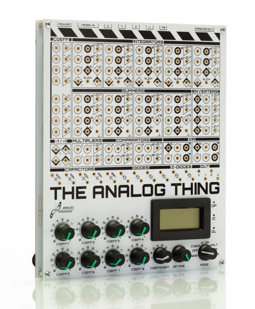
Figure 1 — THAT front panel, showing the patch field with integrators (INT1–INT5), summers (SUM1–SUM4), inverters (INV1–INV4), multipliers (MUL1–MUL2), comparators (CMP1–CMP2), coefficient potentiometers (PT1–PT8), and the mode selector.

THAT BASE PCB — sheet 1

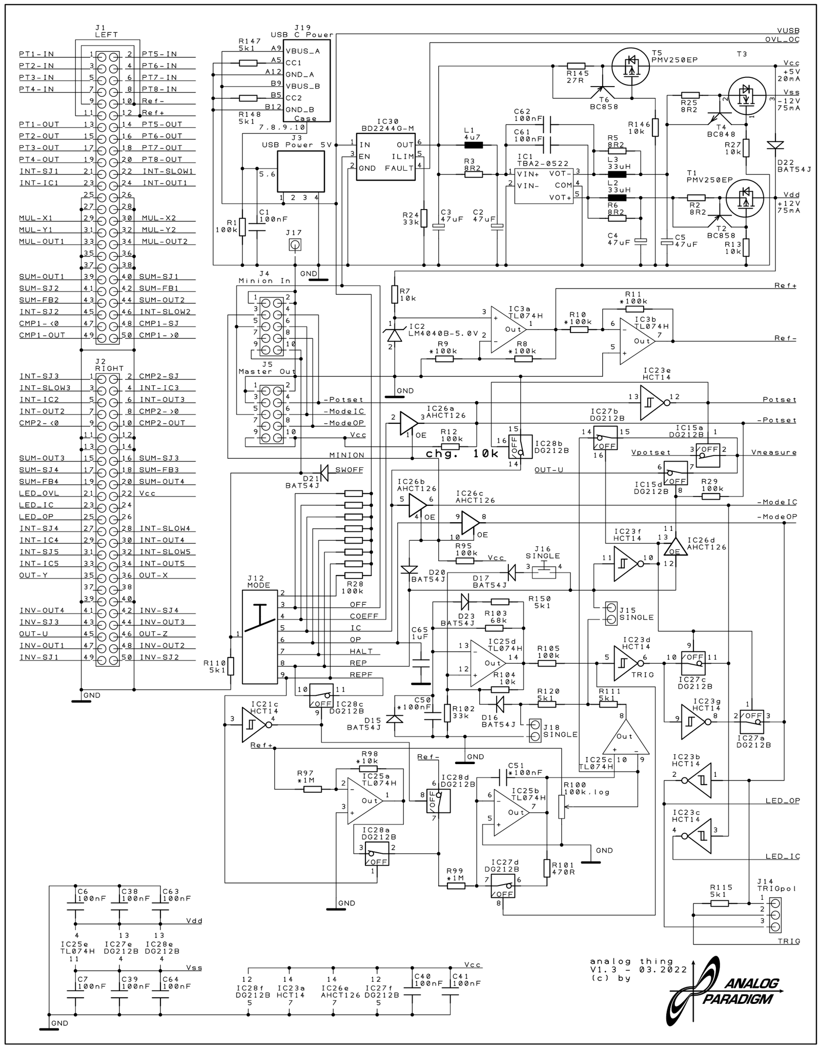
Figure 2 — THAT BASE PCB schematic sheet 1 (v1.3, 2022). Shows the DC/DC converter, HYBRID port, and master/minion inter-board signalling logic.

THAT FRONT PCB — patch field 1

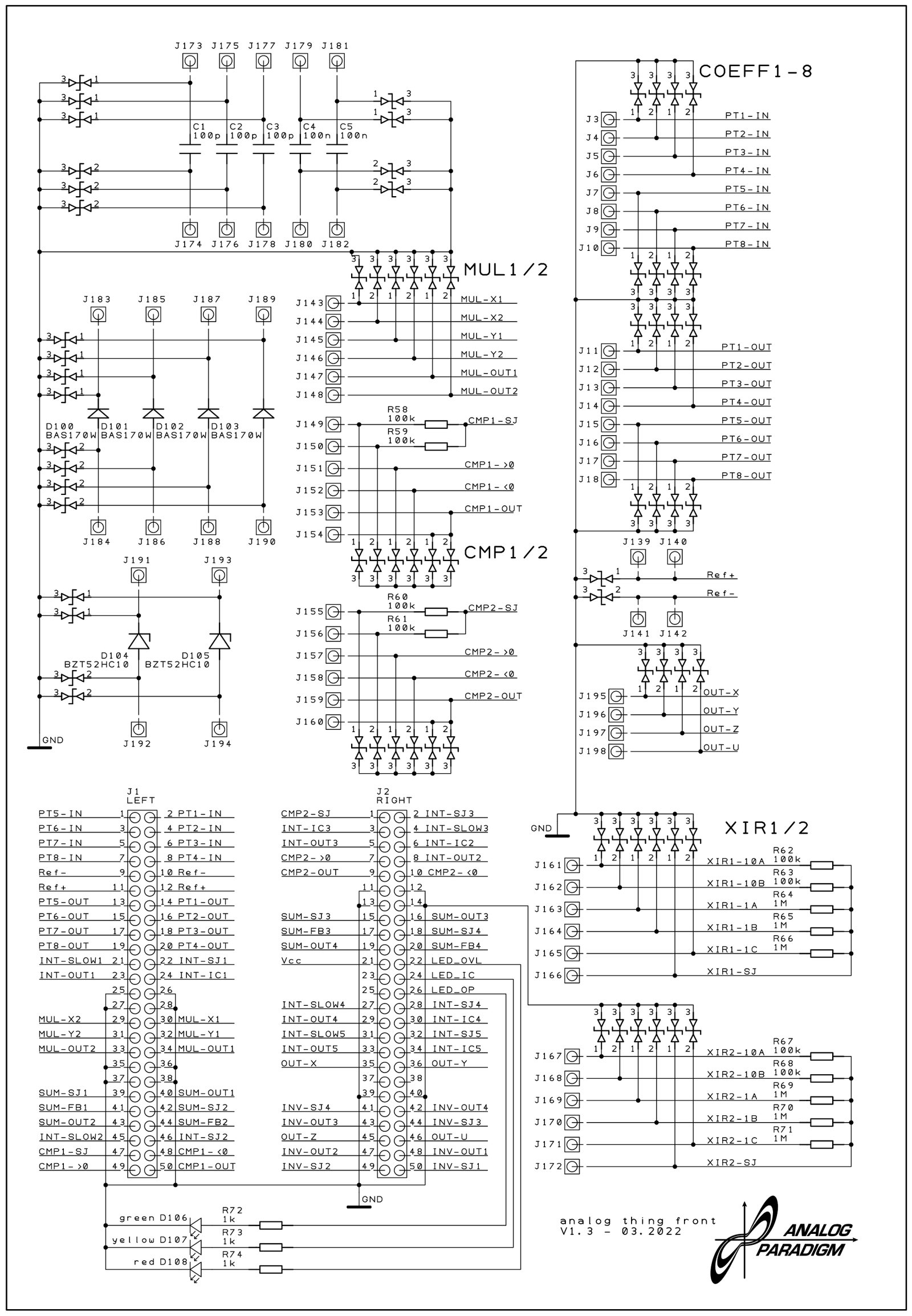
Figure 3 — THAT FRONT PCB schematic sheet 1 (v1.3, 2022). Multipliers MUL1/MUL2, comparators CMP1/CMP2, coefficient potentiometers COEFF1–8, and resistor networks XIR1/2 visible at left.

THAT FRONT PCB — patch field 2

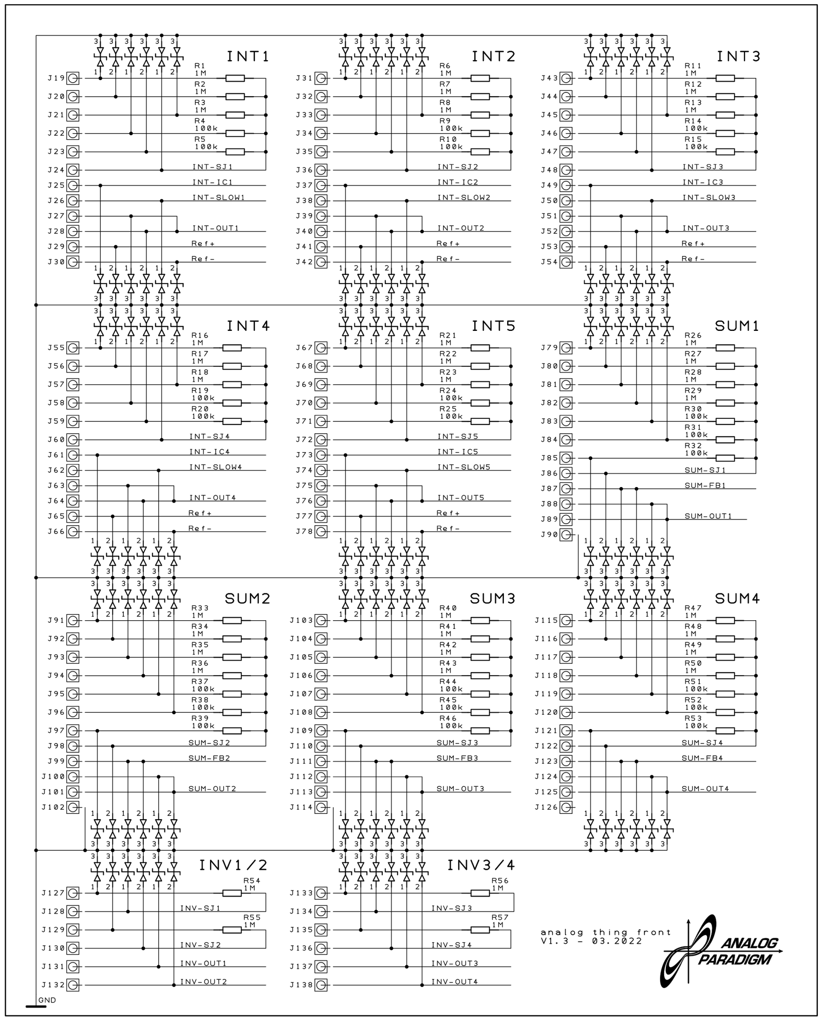
Figure 4 — THAT FRONT PCB schematic sheet 2 (v1.3, 2022). All five integrators (INT1–INT5), all four summers (SUM1–SUM4), and all four inverters (INV1–INV4) with their input resistor networks.

THE Analog Thing — Volume 5 — Worked examples & applications

Introduction — How to Read This Volume

Demo 1 — Simple Harmonic Oscillator (Undamped Pendulum)

Physical system and equations

Scaling

Element inventory for this patch

Coefficient settings

Patch SVG — Signal-flow diagram

Expected output

Demo 2 — Damped Pendulum (Mass-Spring-Damper)

Physical system and equations

Scaling

Element inventory

Coefficient settings

Patch SVG

Expected output and phase portrait

Demo 3 — Lorenz Attractor

Physical system and equations

Scaling

Element inventory

Coefficient settings (starting point)

Patch SVG — Three-loop signal flow

Expected output

Demo 4 — Van der Pol Oscillator

Physical system and equations

Scaling

Element inventory

Coefficient settings (μ = 1, normalised X = x/2)

Patch SVG — Limit-cycle topology

Expected output

Demo 5 — Predator-Prey Dynamics (Lotka-Volterra)

Physical system and equations

Scaling

Element inventory

Coefficient settings

Patch SVG

Expected output

Demo 6 — Euler Spiral (Cornu Spiral / Clothoid)

Physical system and equations

Scaling

Element inventory

Coefficient settings

Patch SVG

Expected output

Demo 7 — Rössler Attractor (Two-THAT Minion Chain)

Physical system and equations

Minion-chain arrangement

Scaling

Coefficient settings (key pots)

Expected output

Newsletter Content Index

Scaling Reference Tables

Table A — Standard normalisation constants used in this volume

Table B — Mode selector quick reference

Table C — Integrator input weighting

Table D — Multiplier sign convention

Table E — Element count vs. demo complexity

Practical Patching Notes

Initial-condition sign convention

Overload recovery

REP vs. REPF mode selection

Coefficient-potentiometer adjustment workflow

Daisy-chain topology for multi-THAT patches

Cross-Reference to Other Volumes

Figure References