THAT — The Analog Thing · Volume 1
THE Analog Thing — Volume 1 — Overview & the modern-analog revival
What THAT is, who built it, why analog returned, and how to decide whether it belongs on the bench — context for Vols 2–8
1.1 About This Volume
This volume is the entry point for the eight-volume THE Analog Thing (THAT) engineer reference series. It establishes the machine’s identity, the industrial and academic context that brought it into existence, and a precise technical profile based on the official First Steps manual (v2.0, 2023) and the Analog Paradigm V1.3 schematics. Readers who need no motivational framing may skip directly to Section 5 (physical tour) or Section 7 (specification table).
1.1.1 Depth Index — The Eight-Volume Series
Table 1 — Depth Index — The Eight-Volume Series
| Vol | Title | Primary Audience |
|---|---|---|
| 1 | Overview & the modern-analog revival (this volume) | All readers; context and orientation |
| 2 | Hardware & architecture | EE / mathematician |
| 3 | Computing elements & patching | All practitioners |
| 4 | Programming | Control / simulation engineer |
| 5 | Worked examples & applications | Scientist / student |
| 6 | Expansion & hybrid | Embedded / systems engineer |
| 7 | Comparison & context | Senior EE / buyer |
| 8 | Cheatsheet | All readers (field reference) |
Note — Cross-references to other volumes appear throughout this text as “see Vol N.” All electrical values cited herein are sourced directly from the First Steps manual or the Analog Paradigm V1.3 schematic set; no values are assumed.
1.2 What THAT Is
THE Analog Thing — universally abbreviated THAT — is a solid-state, desk-top electronic analog computer produced by Anabrid GmbH in Berlin, Germany. It has been in continuous production since approximately 2021. THAT computes by representing quantities as time-varying continuous voltages; the machine unit is the interval −1 to +1, implemented as −10 V to +10 V on the physical hardware. Quantities never take the form of discrete digital symbols: every variable exists as a voltage level at every instant.
THAT is simultaneously a research instrument, an educational platform, and a community object. The First Steps manual describes it as “a high-quality, low-cost, open-source, not-for-profit cutting-edge analog computer.” The machine accepts 2 mm banana-plug patch cables on a front panel and draws power from any USB-C supply — the same charger that powers a smartphone. That combination of laboratory-grade computation and everyday convenience is deliberate: Anabrid designed THAT specifically to lower the entry barrier to analog practice.
1.2.1 Machine Unit and Voltage Rails
The distinction between the abstract machine unit and the physical rail voltage is foundational to programming THAT correctly.
  Abstract domain          Physical domain
  ─────────────────        ─────────────────
      +1  ←────────────→   +10 V   (machine-unit reference)
       0  ←────────────→     0 V   (GND)
      -1  ←────────────→   -10 V   (machine-unit reference)
All patch diagrams, coefficient settings, and scaling calculations in Vols 2–5 operate in the abstract domain. The physical supply rails are ±12 V, generated by an on-board DC/DC converter from the 5 V USB-C input; the ±10 V machine-unit reference is derived from those rails and sets the effective computational boundary. Driving a summing junction beyond ±10 V produces an overload condition signalled by the OL state LED on the front panel.
1.2.2 Computing Paradigm
THAT is a continuous-time, parallel, patch-programmable computer. Unlike a stored-program machine, it has no instruction stream, no clock cycle, and no sequential fetch-decode-execute loop. All computing elements operate simultaneously. The “program” is the physical topology of patch cables connecting element outputs to element inputs. The solution of a differential equation emerges as a voltage waveform in real time the moment the mode selector is placed in OP (operate) mode.
This implies two important characteristics the reader must internalize before proceeding to later volumes:
Note — A THAT patch is not debugged by stepping through code; it is diagnosed by measuring voltages at intermediate jacks with an oscilloscope and reasoning about signal-flow topology (see Vol 4). Patching errors produce wrong waveforms or overloads, not error messages.
Note — Computation speed is set by RC time constants, not by a clock. A first-order integrator with an input of exactly −1 machine unit and initial condition of zero will drive its output from 0 to +1 in exactly 1 ms at normal speed. This is the fundamental time reference for all speed-scaling calculations (see Vol 3).
1.3 Anabrid, Bernd Ulmann, and the Open-Hardware Ethos
1.3.1 Founding and Identity
Anabrid GmbH (Am Stadtpark 3, 12167 Berlin, Germany; [email protected]) was co-founded in 2020 by Professor Dr. Bernd Ulmann, then of Frankfurt. The company name combines “analog” and “hybrid.” Ulmann is the author of Analog and Digital Computer Programming (De Gruyter, available in the THAT community library) and has spent decades preserving, studying, and reviving analog computation. Thomas Fischer co-authored the First Steps manual.
Charles Platt’s 2022 Make magazine article (“Electronics Fun & Fundamentals: Analog Reborn”) quotes Ulmann directly: “Our goal is to bring the idea of analog computing back to the world… We have hobbyists, musicians (controlling analog synthesizers), many students, sometimes large companies.” The article confirmed the retail price at that time at under $350 USD including US shipping.
1.3.2 Open-Hardware Licensing
THAT’s schematics are released under the Analog Paradigm brand and are publicly available. The V1.3 schematic set examined for this series carries the designation “analog thing front / base V1.3 — 03.2022 (c) by Analog Paradigm.” The First Steps manual itself is published under the Creative Commons Attribution-NonCommercial-ShareAlike 4.0 International License (CC BY-NC-SA 4.0), making the documentation legally reproducible for educational use with attribution. The combination of open schematics and open documentation is explicitly intended to support a community of practice rather than to protect intellectual property.
Tip — The community wiki lives at
the-analog-thing.org. The newsletter archive (sixteen issues as of this writing) documents production milestones, user experiments, application notes, and community Q&A. Key milestones from newsletters 1–3: Newsletter #1 announced a TEDx demonstration; Newsletter #2 confirmed V1 entering volume production (100 units initial batch) and noted Version 1 PCBA had entered production; Newsletter #3 reported a second production run with further improvements, and included a user testimonial describing the Lorenz attractor being computed live.
1.3.3 Newsletter Milestones (Issues 1–3)
Table 2 — Newsletter Milestones (Issues 1–3)
| Issue | Key Announcement |
|---|---|
| #1 | THAT introduced publicly; TEDx presentation by Ulmann and Fischer; wiki setup announced; book (Analog and Hybrid Computer Programming) highlighted |
| #2 | V1 PCBA entered production — initial batch of 100 units; ordering page launched; first application note (Lorenz attractor) published |
| #3 | Second production run announced; user testimony on THAT’s accessibility; Lorenz attractor run photographed; ongoing documentation sprint described |
1.4 Why Analog Computing Returned
The re-emergence of practical analog computing in the 2020s is not nostalgia; it is a response to several converging technical and educational pressures that the First Steps manual enumerates explicitly.
1.4.1 Energy Efficiency
Digital processors execute instructions through billions of transistor switching events per second. Each switching event dissipates energy proportional to CV²f (capacitance × rail voltage squared × frequency). Jennifer Hasler’s 2016 IEEE IRPS paper, cited in the First Steps manual, quantifies the opportunity: physical analog computing can, for certain classes of computation, be several orders of magnitude more energy-efficient than CMOS digital. THAT itself consumes only USB bus power — on the order of a few watts — while simultaneously solving coupled differential equations in real time.
Note — The energy argument applies most forcefully to massively parallel, approximate, continuous-value computations — precisely the class dominated by neural inference and dynamical-system simulation. Digital remains preferable for exact integer arithmetic and general-purpose symbolic processing. See Vol 6 for hybrid architectures that exploit both.
1.4.2 Moore’s Law Saturation
Hennessy and Patterson’s Computer Architecture: A Quantitative Approach (6th ed., 2019), cited in the First Steps manual, documents the deceleration of single-thread performance improvements as transistor scaling approaches atomic limits. Hybrid analog-digital architectures represent one credible path to continued performance improvement without requiring further lithographic shrinkage.
1.4.3 Cyber-Physical Security
Daniel Geer’s 2018 Hoover Institution paper, also cited by Ulmann, argues that purely digital infrastructure creates attack surfaces that analog fallback systems can reduce. An analog computer solving a control equation is inherently non-addressable by network-borne software exploits.
1.4.4 Educational and Intellectual Value
George Lang’s 2000 paper in Sound and Vibration frames the intellectual dimension: analog computing demands direct engagement with calculus, differential equations, and physical intuition in a way that black-box digital simulation does not. Patching THAT to solve the mass-spring-damper system (a canonical second-order ODE) requires the operator to derive the equations, scale variables, choose initial conditions, and interpret waveforms — none of which can be delegated to a compiler or numerical solver.
1.4.5 The Hybrid Future
The First Steps manual explicitly anticipates “an analog-digital hybrid computing future.” THAT’s HYBRID port (Section 5 below) is the hardware realization of this vision: it provides a 0–3.3 V logic-level-compatible interface for microcontrollers, enabling Arduino or similar devices to read THAT outputs and write THAT initial conditions or mode-control signals. Platt’s Make article confirmed that the community had already built a data logger and an Arduino-based oscilloscope for THAT within the first year of production.
1.4.6 Dynamical-Systems Education
Differential equations govern the temporal behavior of virtually every physical system of engineering interest: mechanical vibration, chemical kinetics, population biology, epidemiology, electrical circuits, orbital mechanics. THAT provides immediate, visceral access to these dynamics. Adjusting a coefficient potentiometer while watching the Lorenz attractor shift on an oscilloscope is pedagogically distinct from modifying a floating-point parameter in a Python simulation — the feedback is physical and continuous rather than symbolic and discrete.
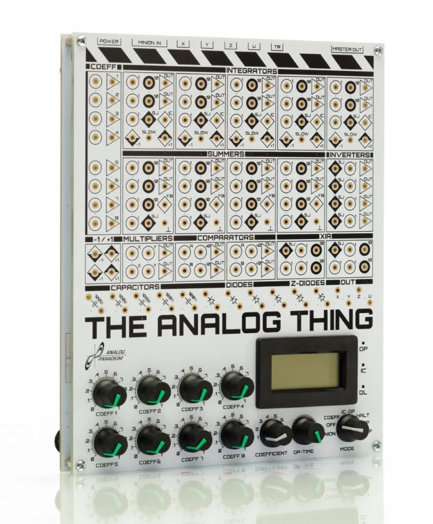
1.5 Physical Tour — Panel, Jacks, and Element Groups
THAT is a single-board instrument approximately the size of a large paperback book. The front panel is the primary user interface; the rear panel carries power and signal connections.
1.5.1 Rear Panel Connections
Table 3 — Rear Panel Connections
| Connector | Function |
|---|---|
| USB-C IN | 5 V power input (USB data pins unused); any USB phone charger suffices |
| MINION IN | Ribbon cable input for daisy-chain multi-THAT expansion |
| MASTER OUT | Ribbon cable output to a subordinate THAT in minion mode |
| RCA Out (X, Y, Z, U) | Four analog outputs, attenuated to ±1 V for audio hardware / software oscilloscopes |
| RCA Trigger Out | REP/REPF trigger pulse for oscilloscope synchronization |
| HYBRID Port | Four channels shifted to 0–3.3 V for microcontroller interfacing |
Note — The RCA Out signals are attenuated copies of whatever is patched into the X, Y, Z, and U output jacks on the front panel. The attenuation makes them safe for audio-input devices; a sound card or USB audio interface can serve as a two-channel oscilloscope (with the caveat that DC and low-frequency components are filtered by the coupling capacitors in the audio path).
1.5.2 Front Panel — Element Groups
The First Steps manual numbers twenty-three distinct panel features. For programming purposes, eight functional groups matter most:
┌─────────────────────────────────────────────────────────────────────┐
│  THAT V1.3 — Functional Panel Map                                   │
├──────────────────┬──────────────────────────────────────────────────┤
│ GROUP            │ LOCATION (approximate, left → right, top → bot.) │
├──────────────────┼──────────────────────────────────────────────────┤
│ Integrators (5)  │ Upper-left quadrant; each has 5 inputs, IC, SLOW │
│ Machine Units    │ Adjacent to integrators; ±1 diamond jacks         │
│ Inverters (4)    │ Lower-left; single-input sign inverters           │
│ Summers (4)      │ Upper-center; 7 inputs each, FB and GND jacks     │
│ Multipliers (2)  │ Center; four-quadrant analog multiplication       │
│ Comparators (2)  │ Center; conditional routing A+B>0 or A+B<0       │
│ Coefficient Pots │ Lower-center; 8 pots, selected via front knob     │
│ Output Jacks     │ Right edge; X, Y, Z, U — routed to RCA rear ports │
├──────────────────┼──────────────────────────────────────────────────┤
│ Resistor Nets    │ XIR blocks; extend summing junctions of any elem. │
│ Capacitors       │ Discrete exposed caps for user-connected RC nets  │
│ Diodes/Zeners    │ Nonlinear elements for clamping, rectification    │
└──────────────────┴──────────────────────────────────────────────────┘
1.5.3 Element Inventory (Verified from First Steps Manual and Schematics)
The following counts are taken directly from the First Steps manual (Section 7) and confirmed against the front-panel schematic (THAT-Front V1.3, sheets 1 and 2):
Table 4 — The following counts are taken directly from the First Steps manual (Section 7) and confirmed against the front-panel schematic (THAT-Front V1.3, sheets 1 and 2)
| Element | Count | Key Parameters |
|---|---|---|
| Integrators | 5 | 5 inputs each (×1 and ×10 weighted); IC input; SLOW jack; sign-inverting; two output jacks per integrator |
| Summers | 4 | 7 inputs each (×1 and ×10 weighted); sign-inverting; FB and GND jacks; two output jacks each |
| Inverters | 4 | Single input; unity-gain sign inversion; two output jacks each |
| Multipliers | 2 | Four-quadrant; two output jacks each |
| Comparators | 2 | Two-input (A, B); output routes either > or < input signal based on sign of A+B |
| Coefficient Potentiometers | 8 | Range 0–1 (one machine unit); readable via panel meter in COEFF mode |
| Machine Unit Jacks | — | +1 and −1 constant voltage references (diamond-shaped jacks) |
| Resistor Networks (XIR) | 2 | Extend summing junctions via SJ-to-SJ connection |
| Output Jacks (X, Y, Z, U) | 4 | Front panel; mirrored to RCA rear outputs |
Note — The integrator input weighting deserves emphasis: two of the five inputs on each integrator are weighted by a factor of 10, providing a signal multiplication at the summing junction without consuming a separate multiplier element. Similarly, three of the seven summer inputs carry ×10 weighting. This is critical for scaling (see Vol 3).
1.5.4 Jack Types and Color/Shape Coding
THAT uses a consistent visual grammar for its jacks. The First Steps manual (Section 8) defines the conventions:
Table 5 — THAT uses a consistent visual grammar for its jacks. The First Steps manual (Section 8) defines the conventions
| Jack Marking | Shape | Meaning |
|---|---|---|
| Filled circle | Round | Input — accepts one signal |
| Triangle | Triangular | Output — can drive multiple inputs via cable stacking |
| Diamond (upper half black) | Diamond | Machine unit +1 constant |
| Diamond (lower half black) | Diamond | Machine unit −1 constant |
| White circle labeled “1” | Round | Unweighted (×1) input |
| Black circle labeled “10” | Round | Weighted (×10) input |
| ”SJ” | Special | Summing junction — interconnects resistor network to element |
| ”IC” | White diamond | Initial condition input for integrator |
| ”SLOW” | Special | Connect integrator output here to reduce speed ×0.01 |
| ”FB” | White diamond | Feedback resistor jack of a summer |
Tip — Multiple patch cable plugs can be physically stacked in a single jack to fan-out one output to several inputs. An input, however, may only receive a single signal — stacking two outputs into one input shorts them together and will likely cause an overload.
1.5.5 The SLOW Connection
The SLOW jack on each integrator deserves special mention because it is a hardware-implemented time-scaling shortcut. Connecting an integrator’s output to its own SLOW input reduces that integrator’s operating speed by a factor of 100 (×0.01 of normal). The practical effect:
Normal speed:    input = -1 MU,  IC = 0  →  output reaches +1 MU in   1 ms
SLOW connected:  input = -1 MU,  IC = 0  →  output reaches +1 MU in 100 ms
This is the simplest way to slow a patch into the visible range without modifying coefficient values. See Vol 3 for full time-scaling methodology.
1.5.6 Modes of Operation
The mode selector knob on the front panel governs THAT’s operating state:
Table 6 — The mode selector knob on the front panel governs THAT's operating state
| Mode | Behavior |
|---|---|
| COEFF | Coefficient-setting mode; selected pot value shown on panel meter (0–1 range) |
| IC | Initial condition phase; integrator outputs driven to (inverted) IC input values |
| OP | Operate; all integrators integrate, patch runs continuously |
| HALT | Integration suspended; all integrator outputs held at last value |
| REP | Repeated IC→OP cycles; OP time set by front-panel pot (0–10 s range); triggers RCA Trigger Out |
| REPF | As REP but 100× faster; OP time 0–100 ms; enables stable oscilloscope display |
| MINION | This THAT follows a master THAT’s control signals over the ribbon cable |
The panel meter serves double duty: in COEFF mode it reads the selected potentiometer output in the 0–1 unit range; in IC, OP, HALT, and MINION modes it reads whatever signal is patched to the U output jack in the ±1 unit range; in REP mode it reads OP time in seconds; in REPF mode it reads OP time in milliseconds.
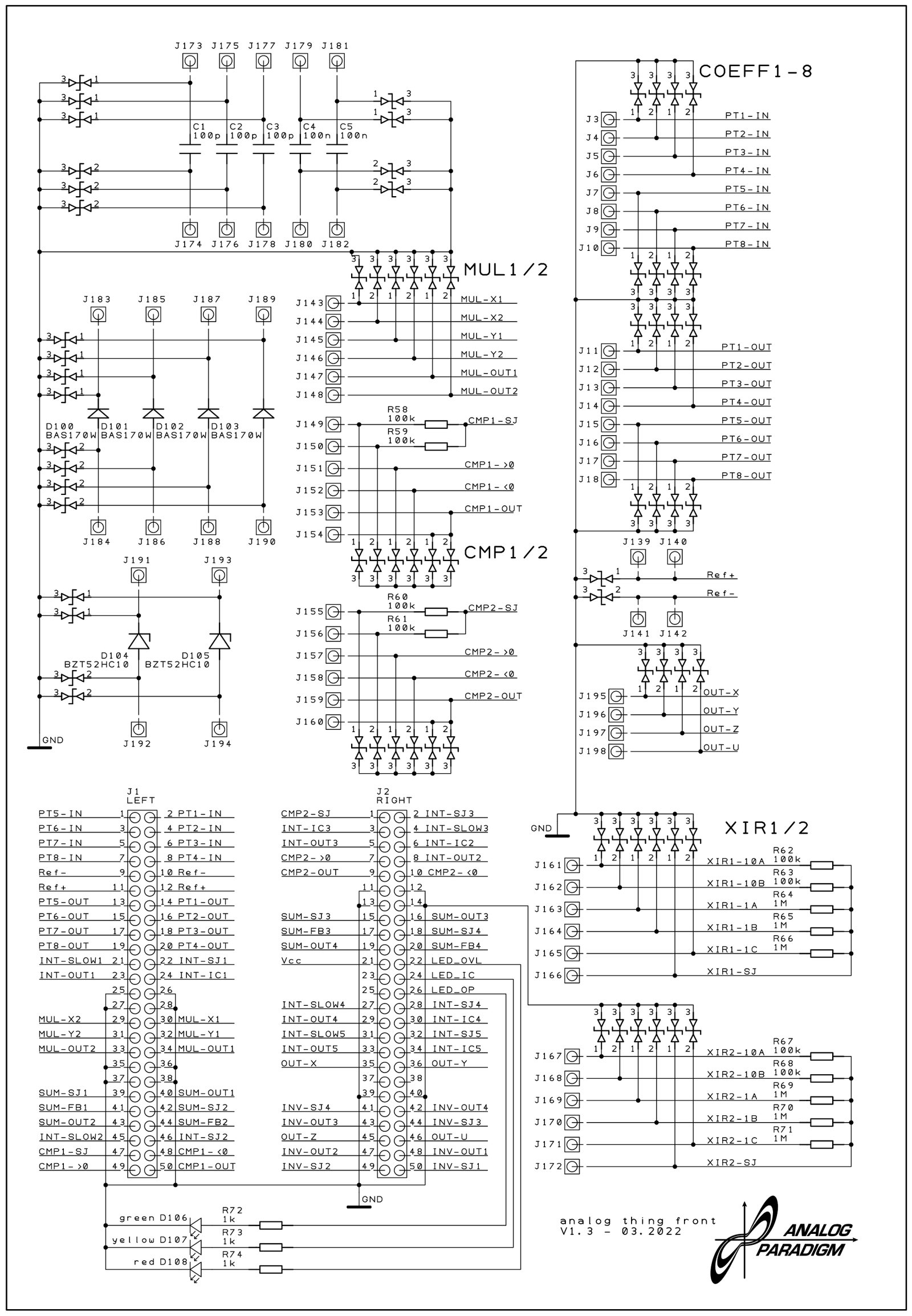
1.5.7 Schematic Architecture Summary (V1.3)
The Analog Paradigm V1.3 schematic set comprises five sheets:
Table 7 — The Analog Paradigm V1.3 schematic set comprises five sheets
| Sheet | Content |
|---|---|
| Base-01 | Power regulation (±12 V rails from DC/DC converter), microcontroller (mode/coefficient control), multiplexer logic |
| Base-02 | Coefficient potentiometers (PT1–PT8), panel meter circuit (TL074H driver), pot selection logic |
| Base-03 | Integrators INT1–INT5 (each built around an op-amp with timing capacitor), Summers SUM1–SUM4, Inverters INV1–INV4 |
| Base-04 | Multipliers MUL1/MUL2, Comparators CMP1/CMP2, overload detection, LED driver, volt measurement |
| Base-05 | Output jacks (X, Y, Z, U), RCA attenuation, HYBRID port level-shift (0–3.3 V), MINION/MASTER ribbon interface, power input (USB-C) |
The front-panel sheets (Front-01, Front-02) document the patch-panel connector grid: all integrator, summer, inverter, multiplier, comparator, resistor network, and coefficient input/output jacks as physical connectors with their net names.
Note — The op-amps used in the integrator and summer stages are TL074H (quad JFET op-amp) devices. The internal supply rails are ±12 V (generated by the DC/DC converter from USB-C 5 V); the ±10 V machine-unit reference is derived from those rails and defines the computational boundary. A separate logic supply powers the digital control circuitry.
1.6 Decision Tree — Is THAT the Right Machine?
THAT is not the only modern analog or hybrid computing option. The following decision tree helps a practitioner place THAT against alternatives.
START — Is the primary goal analog computation or hybrid analog-digital?
│
├─► Analog-only, educational / research, ≤ ~20 computing elements?
│   ├─► Budget under ~$400 USD, desktop form factor? ──────────────► THAT ✓
│   └─► Larger budget, need more elements per board? ─────────────► Consider Anabrid LUCIDAC (chip-based, higher density)
│
├─► Hybrid analog-digital, need microcontroller integration?
│   ├─► Arduino or similar as digital partner, THAT as analog engine? ─► THAT + HYBRID port ✓
│   └─► Need tightly coupled FPGA or DSP? ─────────────────────────► Research-grade hybrid system
│
├─► Purely historical / vintage restoration?
│   └─► Seek Heathkit EC-1, ES-400, EAI TR-10, or similar vintage ──► Not THAT's mission
│
└─► Need more elements than one THAT provides?
    └─► Daisy-chain multiple THATs via MASTER OUT → MINION IN ─────► THAT minion chain ✓
        (no upper limit on chain length per manual)
1.6.1 THAT vs. Comparable Modern Options
Table 8 — THAT vs. Comparable Modern Options
| Criterion | THAT V1.3 | Typical FPAA (e.g., Hasler FPAA dev board) | Vintage EAI TR-10 |
|---|---|---|---|
| Machine unit | ±10 V | ±1–3 V (varies) | ±10 V or ±100 V |
| Integrators | 5 | Configurable (dozens of subcircuits) | 10 |
| Patch method | Physical 2 mm banana jacks | Software (no physical patch) | Physical phone jacks |
| Open-source HW | Yes (CC-licensed schematics) | Partial | No (1960s proprietary) |
| Power | USB-C (5 W class) | USB / wall supply | 115/230 VAC, ~400 W |
| Expansion | Ribbon-cable minion chain | Bus backplane | Separate unit cabinets |
| Price (new) | ~$300–400 USD | $100–300 USD (eval board only) | $500–5000 USD (used, restored) |
| Hybrid port | Yes (0–3.3 V, 4 channels) | Yes (native digital fabric) | No |
| Community / docs | Active (newsletters, wiki) | Academic / sparse | Historical only |
Note — FPAA-based systems offer far greater element density and reconfigurability but eliminate the tactile patch-cable experience that makes THAT particularly effective as a teaching instrument. The physical act of patching forces the operator to reason about signal flow in a way that a GUI-configured FPAA does not.
1.6.2 When THAT Is Not Sufficient
The operator should consider minion expansion or a different platform when:
- More than five integrators are required in a single ODE system (e.g., sixth-order mechanical systems, high-dimensional coupled oscillators).
- Precision better than the inherent ±1% coefficient potentiometer accuracy is required (see Vol 8 on calibration).
- Computation time constants shorter than approximately 1 µs are needed (THAT’s op-amps are TL074H quad JFET devices, not ultra-wideband).
- A fully automated, computer-controlled sweep over many parameter combinations is required without manual pot adjustment.
1.7 Specification Quick-Table
All values sourced from the First Steps manual v2.0 (2023) and Analog Paradigm V1.3 schematics (March 2022) unless noted with †.
Table 9 — Specification Quick-Table
| Parameter | Value | Source |
|---|---|---|
| Machine unit | ±1 (abstract) = ±10 V (physical reference) | First Steps §5 |
| Internal supply rails | ±12 V (DC/DC converter from USB-C 5 V) | First Steps FAQ; Schematic Base-01 |
| Power input | USB-C 5 V (USB data unused) | First Steps §2; Base-05 |
| Integrators | 5 | First Steps §7 |
| Inputs per integrator | 5 (two weighted ×10, three ×1) | First Steps §7; Front-02 |
| IC input per integrator | 1 | First Steps §7 |
| SLOW jack per integrator | 1 (connects output to self, reduces speed ×0.01) | First Steps §8 |
| Normal integration rate | 1 ms to traverse full machine unit at input = −1 MU | First Steps §8 |
| SLOW integration rate | 100 ms to traverse full machine unit at input = −1 MU | First Steps §8 |
| Summers | 4 | First Steps §7 |
| Inputs per summer | 7 (three weighted ×10, four ×1) | First Steps §7 |
| Inverters | 4 | First Steps §7 |
| Multipliers | 2 | First Steps §7 |
| Comparators | 2 | First Steps §7 |
| Coefficient potentiometers | 8 | First Steps §7 |
| Coefficient pot range | 0–1 (one machine unit) | First Steps §5 |
| Machine unit reference jacks | +1 and −1 | First Steps §8 |
| Resistor networks (XIR) | 2 | First Steps §8; Front-01 |
| Output jacks (X, Y, Z, U) | 4 | First Steps §7 |
| RCA outputs | 4 (X, Y, Z, U), attenuated to ±1 V | First Steps §7 |
| RCA trigger output | 1 (REP/REPF synchronization) | First Steps §7 |
| HYBRID port channels | 4, shifted to 0–3.3 V | First Steps §7; Base-05 |
| MINION expansion | Unlimited chain via ribbon cable | First Steps §7 |
| REP mode OP time | 0–10 s (set by front-panel pot) | First Steps §7 |
| REPF mode OP time | 0–100 ms (100× faster than REP) | First Steps §7 |
| Panel meter range (COEFF) | 0–1 unit | First Steps §7 |
| Panel meter range (OP/IC/HALT) | ±1 unit (reads U jack) | First Steps §7 |
| Panel meter range (REP) | 0–10 s | First Steps §7 |
| Panel meter range (REPF) | 0–100 ms | First Steps §7 |
| Patch cable type | 2 mm banana plug (30 cables included) | First Steps §3 |
| State LEDs | OP (running), IC (initial condition), OL (overload) | First Steps §7 |
| Schematic version | V1.3, March 2022 | Schematic title block |
| Manual version | First Steps v2.0, 2023 | Manual title page |
| License (manual) | CC BY-NC-SA 4.0 | Manual copyright page |
| Manufacturer | Anabrid GmbH, Berlin, Germany | Manual; anabrid.com |
| Retail price at launch (approx.) | <$350 USD including US shipping† | Make magazine, Dec. 2022 |
Tip — The schematic version (V1.3) and manual version (v2.0) are not directly synchronized — the schematics predate the manual revision. When resolving any discrepancy between schematic and manual, treat the schematic as the ground truth for electrical values and the manual as the ground truth for panel labeling and operational procedures.
1.8 Signal-Flow Convention
The following SVG diagram illustrates the fundamental building block of any THAT patch: an integrator in a feedback loop. This is the smallest possible complete computation — a first-order linear ODE.
Figure — Canonical first-order feedback patch on THAT. A coefficient potentiometer scales the input; the integrator inverts and integrates; the output feeds back to close the loop. This is the radioactive decay patch: N’ = −λN.
1.9 Further Reading and Community Resources
Table 10 — Further Reading and Community Resources
| Resource | Location / Reference |
|---|---|
| First Steps manual (primary) | Shipped with THAT; PDF at the-analog-thing.org/docs |
| Analog and Hybrid Computer Programming | Bernd Ulmann; De Gruyter (available via community library) |
| THAT wiki | the-analog-thing.org |
| Newsletter archive | the-analog-thing.org (issues 1–16 as of this writing) |
| Schematics (V1.3) | Analog Paradigm; redistributed in this project under open-hardware terms |
| Make “Analog Reborn” (Platt, 2022) | makezine.com; reproduced in hub Library |
| Anabrid GmbH shop | shop.anabrid.com |
| Community Facebook group | Mentioned in First Steps manual and Make article |
| Jennifer Hasler (2016) energy paper | IEEE IRCS 2016, San Diego |
Subsequent volumes in this series drill into each functional group and technique in the depth appropriate to a working engineer. Vol 2 begins with the integrator as the fundamental computing element — its op-amp implementation, timing analysis, IC behavior, and overload recovery — and proceeds through summers, inverters, and the resistor network extension mechanism.
Comments (0)