Heathkit ES-400 · Volume 6
Heathkit ES-400 — Volume 6 — Sample programs & demonstrations
Six worked demonstrations from grade-school integrator to college-depth damped oscillator, predator-prey, and projectile — each with scaling derivation, patch diagram, pot-setting table, and expected waveform
6.1 Preface — How to Use This Volume
This volume is a practical laboratory companion. Each demonstration is self-contained: the physical equation is stated, amplitude and time scaling are derived, the patch is described in both prose and an inline SVG block-diagram, coefficient-pot settings are tabulated, and the expected output waveform is characterised. The operator is assumed to have the ES-400 powered, all fifteen ES-201 amplifiers balanced, and a dual-channel oscilloscope connected in XY mode at the OSCILLOSCOPE OUTPUT jacks on the front panel.
Two complexity tiers are provided deliberately. The first demonstration (§1) is pitched at a general audience — a classroom visitor, a student seeing the machine for the first time, or an educator who needs a convincing display in under two minutes. Demonstrations §2 through §6 assume a working knowledge of ordinary differential equations, Laplace transforms, and basic circuit analysis at the level of a second- or third-year undergraduate electrical or mechanical engineering programme.
For derivations of the ES-201 amplifier gain, integrator time constant, and coefficient-pot topology, see Vol 2 (hardware & architecture). For scaling theory and programming methodology, see Vol 5 (programming). For physical restoration and balancing of each ES-201, see Vol 4 (acquisition & restoration).
Note — All voltages in this volume are machine voltages. The ES-400 operates at a ±100 V signal range. The ES-2 power supply (see Vol 2) provides the regulated ±250 V plate supply, −450 V grid-bias supply, and 6.3 VAC heater supply required by the ES-201 modules. The ±100 V reference bus (ES-50) supplies the coefficient reference rail and all initial-condition (IC) supplies. Never connect an external signal source to the front panel without first attenuating it to the ±100 V range.
Note — Resistor and capacitor values quoted below are for the passive computing elements — the plug-in components that the operator inserts into the ES-201 jack pairs on the front panel. They are not component values internal to the ES-201 module. The ES-201 itself presents a summing junction whose effective input impedance depends on which plug-in resistors are inserted; see Vol 2 §3 for the complete model.
6.2 Programming Conventions Recap
Before entering the worked examples a brief recap of conventions (full treatment in Vol 4) anchors the notation used throughout this volume.
6.2.1 Machine Reference Values
Table 1 — Machine Reference Values
| Quantity | Symbol | Value |
|---|---|---|
| Full-scale machine voltage | M | ±100 V |
| ES-201 open-loop gain | A | ~50,000 |
| ES-201 output current limit | — | 10 mA |
| Standard integrating RC (1 MΩ + 1 µF) | τ | 1.000 s |
| Standard integrating RC (1 MΩ + 0.1 µF) | τ | 0.100 s |
| Standard summing gain (1 MΩ in / 1 MΩ fb) | — | −1.000 |
| Standard summing gain (1 MΩ in / 2 MΩ fb) | — | −2.000 |
| Coefficient-pot range | — | 0.000 – 1.000 |
| Auxiliary 10-turn pot range | — | 0.00 – 10.00 |
6.2.2 Amplitude Scale Factor
Define a problem variable x (with physical units) and its machine representation X (volts):
X = (M / x_max) × xChoose x_max so that X never exceeds ±100 V during the solution. The scale factor a = M / x_max V per unit.
6.2.3 Time Scale Factor
Define machine time τ_m relative to problem time t:
t = β × τ_mwhere β > 1 slows the solution (useful when the physical process is faster than the oscilloscope can display) and β < 1 speeds it up. Slowing is achieved by increasing all integrator RC time constants by the factor β; speeding up reduces them. For repetitive display at the ES-505 oscillator frequency (0.6–6 Hz), choose β so that one complete solution cycle falls within the oscillator period (typically 0.2–1.5 s).
6.2.4 Amplifier Numbering and Notation
Amplifiers on the front panel are identified A1 through A15. The panel layout places A1–A5 in the top row (left to right), A6–A10 in the middle row, and A11–A15 in the bottom row. Throughout this volume:
- INT denotes an amplifier wired as an integrator (capacitor feedback).
- SUM denotes an amplifier wired as a summer/inverter (resistor feedback).
- Px denotes coefficient potentiometer x (P1–P30 are the standard single-turn pots; P31–P32 are the auxiliary 10-turn pots).
The front panel meter (DC milliammeter) reads zero when its input jack is grounded; it is most useful for slow-running problems. For repetitive mode, the oscilloscope is the correct display device.
6.3 Demo 1 — Integrator as an Accumulator (Grade-School Level)
6.3.1 Objective
Demonstrate in under two minutes — without mathematics — that the integrator accumulates a constant input into a linearly growing output. This is the single most effective introduction for a general audience because the meter needle moves visibly and the behaviour is immediately intuitive.
6.3.2 Equipment Required
- 1 × ES-201 (A1), wired as integrator
- 1 × plug-in input resistor: 1 MΩ
- 1 × plug-in feedback capacitor: 1 µF
- 1 × coefficient potentiometer P1 (single-turn, dial 0–100)
- 1 patch cord from ES-50 +100 V bus to P1 input
- 1 patch cord from P1 output (wiper) to A1 input jack
- 1 patch cord from A1 output to front-panel METER jack
No oscilloscope is required — the front-panel milliammeter serves as output display.
6.3.3 The Mathematics (hidden from the audience)
With input resistor R = 1 MΩ and feedback capacitor C = 1 µF, the integrator time constant τ = RC = 1.000 s. The reference voltage applied through the pot is:
V_in = P1_setting × (+100 V)The integrator output is:
V_out(t) = −(1/τ) ∫₀ᵗ V_in dτ = −(P1/1.0) × t × 100 V/sAt P1 = 0.10 (dial roughly 10/100), the output ramps at −10 V/s. Full scale (100 V) is reached in 10 seconds. At P1 = 0.50 the ramp reaches full scale in 2 seconds.
Because the NE-51 neon overload indicator on A1 illuminates at output saturation, the audience sees the needle slam to full scale and the neon flash — a dramatic visual cue that the computer has “run out of room.”
6.3.4 Patch Diagram
<svg xmlns="http://www.w3.org/2000/svg" width="520" height="180" font-family="monospace" font-size="13">
  <!-- ES-50 Reference bus -->
  <rect x="10" y="60" width="80" height="40" rx="5" fill="#d4e8ff" stroke="#336"/>
  <text x="50" y="76" text-anchor="middle" font-size="11">ES-50</text>
  <text x="50" y="90" text-anchor="middle" font-size="11">+100 V</text>

  <!-- Pot P1 -->
  <rect x="130" y="55" width="60" height="50" rx="5" fill="#fff8cc" stroke="#663"/>
  <text x="160" y="76" text-anchor="middle" font-size="11">P1</text>
  <text x="160" y="90" text-anchor="middle" font-size="11">0–1.0</text>

  <!-- Integrator A1 -->
  <rect x="240" y="45" width="100" height="70" rx="5" fill="#e8ffe8" stroke="#363"/>
  <text x="290" y="68" text-anchor="middle" font-size="11">A1</text>
  <text x="290" y="82" text-anchor="middle" font-size="11">INT</text>
  <text x="290" y="96" text-anchor="middle" font-size="9">1MΩ / 1µF</text>
  <text x="290" y="108" text-anchor="middle" font-size="9">τ = 1.0 s</text>

  <!-- Meter -->
  <rect x="390" y="60" width="80" height="40" rx="5" fill="#ffe8d4" stroke="#633"/>
  <text x="430" y="76" text-anchor="middle" font-size="11">METER</text>
  <text x="430" y="90" text-anchor="middle" font-size="11">mA</text>

  <!-- Connections -->
  <line x1="90" y1="80" x2="130" y2="80" stroke="#333" stroke-width="2"/>
  <line x1="190" y1="80" x2="240" y2="80" stroke="#333" stroke-width="2"/>
  <line x1="340" y1="80" x2="390" y2="80" stroke="#333" stroke-width="2"/>

  <!-- Labels -->
  <text x="108" y="73" text-anchor="middle" font-size="10" fill="#555">ref</text>
  <text x="214" y="73" text-anchor="middle" font-size="10" fill="#555">V_in</text>
  <text x="365" y="73" text-anchor="middle" font-size="10" fill="#555">V_out</text>

  <!-- IC switch label -->
  <text x="290" y="140" text-anchor="middle" font-size="10" fill="#555">IC switch on A1 → RUN to start ramp</text>
</svg>
6.3.5 Pot Settings and Expected Behaviour
Table 2 — Pot Settings and Expected Behaviour
| P1 Dial | V_in to A1 | Ramp Rate (V/s) | Time to Full Scale |
|---|---|---|---|
| 0.00 | 0 V | 0 | — (no movement) |
| 0.05 | 5 V | 5 | 20 s |
| 0.10 | 10 V | 10 | 10 s |
| 0.20 | 20 V | 20 | 5 s |
| 0.50 | 50 V | 50 | 2 s |
| 1.00 | 100 V | 100 | 1 s |
6.3.6 Running the Demonstration
- Set all IC switches to IC. Confirm the meter reads zero.
- Set P1 to approximately 0.10 (dial reading 10).
- Flip A1’s IC switch to OPERATE (RUN). The meter needle begins a steady rise.
- Flip back to IC to reset. Immediately flip to RUN again — the needle rises from zero every time.
- Increase P1 to 0.50 — the needle rises five times faster.
- Explain: “A constant number goes in; a growing ramp comes out. That is exactly what integration means — counting up a steady stream of small increments over time.”
Note — The output sign is negative (the integrator inverts). If the meter is wired through P1 from the ES-50 positive rail, the needle deflects downward. To show upward deflection, either use the −100 V reference bus on the input, or insert one SUM inverter stage between A1 output and the meter.
6.4 Demo 2 — Free-Fall Under Gravity (General-Audience / High-School)
6.4.1 Physical Problem
A body released from rest at height h₀ falls under gravity with no air resistance. The equation of motion is:
ÿ = −g y(0) = h₀, ẏ(0) = 0where y is height (positive upward), g = 9.81 m/s² (or, in the inch-pound system used by most 1950s American engineering textbooks, g = 386 in/s²). The analytic solution is:
y(t) = h₀ − ½ g t²6.4.2 Amplitude and Time Scaling
Choose h₀ = 100 m as the maximum height (a representative building or drop-test height). Then:
amplitude scale:  a_y = 100 V / 100 m = 1 V/m
machine variable: Y = a_y × y = 1 × y  [V, where y is in metres]
For velocity, the maximum speed attained when falling from 100 m is v_max = √(2 g h₀) = √(2 × 9.81 × 100) ≈ 44.3 m/s. Choose:
a_v = 100 V / 50 m/s = 2 V/(m/s)
machine variable: V = 2 × ẏ  [V]
(The 50 m/s denominator gives headroom; actual peak is ~44.3 m/s → 88.6 V, safely within ±100 V.)
For time, the fall duration from 100 m is t_fall = √(2 h₀ / g) ≈ 4.52 s. To display this on a 1-s oscilloscope sweep, choose a time scale factor β = 4 (machine time runs 4× faster than real time):
τ_m = t / β = t / 4This is achieved by using 0.25 µF feedback capacitors in the integrators (reducing τ from 1.0 s to 0.25 s) while keeping the 1 MΩ input resistors.
6.4.3 Scaled Differential Equations
After scaling, the machine equation becomes (derivation in full in Vol 4 §5):
d²Y/dτ_m² = −β² × (a_y / a_y) × g
           = −16 × 9.81
           = −156.96 V/s²  [machine volts per machine second²]
Expressed as a fraction of the ±100 V range: −156.96 / 100 ≈ −1.57. Because a standard integrator with 1 MΩ / 0.25 µF has a gain of −4 per second (i.e., produces 4 V of output ramp per volt of constant input per machine second), the required pot setting for the gravity term is:
P_g = 156.96 / (100 × 4 × 4) = 156.96 / 1600 ≈ 0.098This is consistent with the Research Guide value cited in §8: “Pot 1 → 0.098 (representing g in scaled units).“
6.4.4 Block Diagram and Patch
The patch uses two integrators (A1 as INT-1 computing −V from Ÿ, A2 as INT-2 computing Y from −V), and one summer/inverter (A3) to obtain +V from −V for monitoring and for the feedback path.
<svg xmlns="http://www.w3.org/2000/svg" width="620" height="260" font-family="monospace" font-size="12">
  <!-- Reference supply -->
  <rect x="10" y="95" width="70" height="50" rx="4" fill="#d4e8ff" stroke="#336"/>
  <text x="45" y="113" text-anchor="middle" font-size="10">ES-50</text>
  <text x="45" y="127" text-anchor="middle" font-size="10">+100 V</text>
  <text x="45" y="140" text-anchor="middle" font-size="10">ref</text>

  <!-- Pot P1 (gravity) -->
  <rect x="108" y="100" width="55" height="40" rx="4" fill="#fff8cc" stroke="#663"/>
  <text x="135" y="116" text-anchor="middle" font-size="10">P1</text>
  <text x="135" y="130" text-anchor="middle" font-size="10">0.098</text>

  <!-- Summer A3 (input summer for gravity) -->
  <rect x="200" y="80" width="80" height="70" rx="4" fill="#f0e8ff" stroke="#636"/>
  <text x="240" y="103" text-anchor="middle" font-size="10">A3  SUM</text>
  <text x="240" y="117" text-anchor="middle" font-size="10">1MΩ/1MΩ</text>
  <text x="240" y="131" text-anchor="middle" font-size="10">gain = −1</text>
  <text x="240" y="145" text-anchor="middle" font-size="10">(inverter)</text>

  <!-- INT-1: A1 -->
  <rect x="320" y="75" width="90" height="80" rx="4" fill="#e8ffe8" stroke="#363"/>
  <text x="365" y="98" text-anchor="middle" font-size="10">A1  INT-1</text>
  <text x="365" y="112" text-anchor="middle" font-size="10">1MΩ / 0.25µF</text>
  <text x="365" y="126" text-anchor="middle" font-size="10">τ = 0.25 s</text>
  <text x="365" y="140" text-anchor="middle" font-size="10">out = −Ẏ/a</text>

  <!-- INT-2: A2 -->
  <rect x="448" y="75" width="90" height="80" rx="4" fill="#e8ffe8" stroke="#363"/>
  <text x="493" y="98" text-anchor="middle" font-size="10">A2  INT-2</text>
  <text x="493" y="112" text-anchor="middle" font-size="10">1MΩ / 0.25µF</text>
  <text x="493" y="126" text-anchor="middle" font-size="10">τ = 0.25 s</text>
  <text x="493" y="140" text-anchor="middle" font-size="10">out = Y</text>

  <!-- Oscilloscope output -->
  <rect x="565" y="95" width="50" height="40" rx="4" fill="#ffe8d4" stroke="#633"/>
  <text x="590" y="111" text-anchor="middle" font-size="9">SCOPE</text>
  <text x="590" y="125" text-anchor="middle" font-size="9">Y(t)</text>

  <!-- Connections: ref to P1 -->
  <line x1="80" y1="120" x2="108" y2="120" stroke="#333" stroke-width="1.5"/>
  <!-- P1 to A3 input -->
  <line x1="163" y1="120" x2="200" y2="115" stroke="#333" stroke-width="1.5"/>
  <!-- A3 to A1 input -->
  <line x1="280" y1="115" x2="320" y2="115" stroke="#333" stroke-width="1.5"/>
  <!-- A1 to A2 -->
  <line x1="410" y1="115" x2="448" y2="115" stroke="#333" stroke-width="1.5"/>
  <!-- A2 to scope -->
  <line x1="538" y1="115" x2="565" y2="115" stroke="#333" stroke-width="1.5"/>

  <!-- Feedback: A2 output (Y) loops back to A3 input for IC provision -->
  <!-- Draw feedback arc below -->
  <path d="M538,135 Q540,210 310,210 Q200,210 200,150" stroke="#c33" stroke-width="1.5" fill="none" stroke-dasharray="5,3"/>
  <text x="370" y="225" text-anchor="middle" font-size="9" fill="#c33">Feedback: Y → A3 (for IC only; no active fb in free-fall)</text>

  <!-- IC supply label -->
  <text x="365" y="185" text-anchor="middle" font-size="9" fill="#336">IC on A1: set initial velocity = 0</text>
  <text x="493" y="185" text-anchor="middle" font-size="9" fill="#336">IC on A2: set Y(0) = +100 V (= h₀)</text>

  <!-- Signal labels -->
  <text x="300" y="108" text-anchor="middle" font-size="9" fill="#555">Ÿ</text>
  <text x="430" y="108" text-anchor="middle" font-size="9" fill="#555">−Ẏ/a</text>
  <text x="556" y="108" text-anchor="middle" font-size="9" fill="#555">Y</text>
</svg>
6.4.5 Patch Instructions
- Insert 1 MΩ plug-in resistor at A3 input jack and 1 MΩ plug-in resistor at A3 feedback jack (gain = −1, inverter).
- Insert 1 MΩ plug-in resistor at A1 input jack and 0.25 µF plug-in capacitor at A1 feedback jack.
- Insert 1 MΩ plug-in resistor at A2 input jack and 0.25 µF plug-in capacitor at A2 feedback jack.
- Connect ES-50 +100 V reference → P1 input jack.
- Connect P1 wiper → A3 input jack.
- Connect A3 output → A1 input jack (patching the gravity term into INT-1).
- Connect A1 output → A2 input jack.
- Connect A2 output → oscilloscope vertical (Y channel).
- Connect ES-505 repetitive oscillator output → both A1 and A2 IC input jacks (to reset each cycle).
6.4.6 Coefficient-Pot Settings Table
Table 3 — Coefficient-Pot Settings Table
| Pot | Signal | Setting | Derivation |
|---|---|---|---|
| P1 | Gravity term g | 0.098 | β² g / (M × (1/τ_m)²) = 16 × 9.81 / (100 × 16) ≈ 0.098 |
| A2 IC supply | Initial height h₀ | +100 V (full reference) | h₀ = 100 m → Y(0) = 1 V/m × 100 m = 100 V |
| A1 IC supply | Initial velocity | 0 V | Body starts from rest |
6.4.7 Expected Output
The oscilloscope trace on the Y channel shows a downward-opening parabola starting at +100 V and reaching 0 V at τ_m ≈ 1.13 machine seconds (corresponding to real-time t ≈ 4.52 s). The trace resets automatically at the ES-505 repetitive frequency (set to approximately 1 Hz). At 0.8 Hz repetition, the falling-body curve is continuously displayed as a stable trace.
Note — Because the solution contains no feedback path (free-fall is an open-loop integration), the amplifiers do not sustain oscillation. The solution simply ramps until the IC reset fires. If the repetition rate is set too low, the integrator output will saturate (hit −100 V) and the NE-51 overload lamp on A2 will flash. Increase the repetition frequency or reduce the IC voltage to avoid saturation.
6.5 Demo 3 — Simple Harmonic Oscillator (College — Second-Order Undamped)
6.5.1 Physical Problem
The undamped simple harmonic oscillator governs a mass on a frictionless spring, a lossless LC tank circuit, a simple pendulum at small angles, and many other physical systems:
ÿ + ω₀² y = 0 y(0) = A, ẏ(0) = 0The analytic solution is y(t) = A cos(ω₀ t). The angular frequency ω₀ = 2πf₀, where f₀ is the oscillation frequency. The ES-400 generates a pure sinusoid continuously — the circuit is, in effect, a precision voltage-controlled oscillator.
The operational manual (page 5, Figure 3) shows precisely this configuration as the canonical first example of analog computer programming, using the spring-mass-damper form and noting that “the mass M is connected to the spring with elastic constant K.”
6.5.2 Amplitude Scaling
Set amplitude A = 100 V (full scale). Since the system is undamped, the amplitude never grows, so no headroom margin is needed. Machine variable: Y = y (no scaling required when A = 100 V is chosen as the unit amplitude).
For velocity: ẏ_max = ω₀ A. Choose the pot setting for ω₀² so that the velocity output does not exceed 100 V:
Ẏ_max = ω₀ × 100 V ≤ 100 V → ω₀ ≤ 1 rad/s (for direct machine coupling)For ω₀ > 1 rad/s, reduce the amplitude initial condition or add a scale factor. Typical demonstrations use ω₀ in the range 0.1–2 rad/s, corresponding to f₀ in the range 0.016–0.32 Hz, visible on the front-panel meter.
For oscilloscope display via the ES-505 repetitive oscillator (0.6–6 Hz), higher frequency is preferred. Set:
β = 1/ω₀ (time compression factor)so that one full oscillation cycle corresponds to 2π machine seconds = 6.28 s — too slow for repetitive display. Instead, set ω₀² via the coefficient pot to yield the desired display frequency as follows.
With 1 MΩ / 1 µF integrators (τ = 1 s), the angular frequency of oscillation equals √(P_ω) rad per machine second, where P_ω is the coefficient-pot setting feeding ω₀²:
f_display = √(P_ω) / (2π) [Hz]To display at 1 Hz: P_ω = (2π)² / 1 = 39.5 — exceeds the pot range (max = 1). Use the auxiliary 10-turn pot P31 (range 0–10) in conjunction with a summing gain: P31 set to 3.95 with A3 providing gain of 10 (1 MΩ input / 10 MΩ feedback — use 2-MΩ resistors in parallel for a practical 10 MΩ equivalent), yielding an effective ω₀² of 39.5. Alternatively, reduce τ by using 0.1 µF capacitors (τ = 0.1 s), which multiplies the effective ω₀ by ten, and then set the pot to P = (2π × 0.1)² ≈ 0.395.
For the worked example below, τ = 0.1 s capacitors are specified.
6.5.3 Patch Diagram
<svg xmlns="http://www.w3.org/2000/svg" width="640" height="300" font-family="monospace" font-size="12">
  <!-- INT-1: A1 -->
  <rect x="80" y="100" width="100" height="80" rx="4" fill="#e8ffe8" stroke="#363"/>
  <text x="130" y="123" text-anchor="middle" font-size="11">A1  INT-1</text>
  <text x="130" y="138" text-anchor="middle" font-size="10">1MΩ / 0.1µF</text>
  <text x="130" y="152" text-anchor="middle" font-size="10">τ = 0.1 s</text>
  <text x="130" y="166" text-anchor="middle" font-size="10">out = −ẏ (scaled)</text>

  <!-- INT-2: A2 -->
  <rect x="270" y="100" width="100" height="80" rx="4" fill="#e8ffe8" stroke="#363"/>
  <text x="320" y="123" text-anchor="middle" font-size="11">A2  INT-2</text>
  <text x="320" y="138" text-anchor="middle" font-size="10">1MΩ / 0.1µF</text>
  <text x="320" y="152" text-anchor="middle" font-size="10">τ = 0.1 s</text>
  <text x="320" y="166" text-anchor="middle" font-size="10">out = +y</text>

  <!-- Pot P1: omega squared -->
  <rect x="320" y="220" width="80" height="40" rx="4" fill="#fff8cc" stroke="#663"/>
  <text x="360" y="236" text-anchor="middle" font-size="10">P1  ω₀²</text>
  <text x="360" y="250" text-anchor="middle" font-size="10">0.395</text>

  <!-- Scope outputs -->
  <rect x="460" y="95" width="70" height="35" rx="4" fill="#ffe8d4" stroke="#633"/>
  <text x="495" y="109" text-anchor="middle" font-size="10">SCOPE X</text>
  <text x="495" y="122" text-anchor="middle" font-size="10">−ẏ (cos)</text>

  <rect x="460" y="150" width="70" height="35" rx="4" fill="#ffe8d4" stroke="#633"/>
  <text x="495" y="164" text-anchor="middle" font-size="10">SCOPE Y</text>
  <text x="495" y="177" text-anchor="middle" font-size="10">y (sin)</text>

  <!-- Connections A1 to A2 -->
  <line x1="180" y1="130" x2="270" y2="130" stroke="#333" stroke-width="1.5"/>
  <text x="225" y="122" text-anchor="middle" font-size="9" fill="#555">−ẏ</text>

  <!-- A2 to scopes -->
  <line x1="370" y1="130" x2="460" y2="112" stroke="#333" stroke-width="1.5"/>
  <line x1="370" y1="140" x2="460" y2="167" stroke="#333" stroke-width="1.5"/>

  <!-- A1 to scope X -->
  <line x1="180" y1="120" x2="460" y2="112" stroke="#999" stroke-width="1" stroke-dasharray="4,3"/>

  <!-- Feedback: A2 output (y) through P1 back to A1 input -->
  <path d="M370,150 Q420,150 420,240 Q420,260 360,260" stroke="#c33" stroke-width="1.5" fill="none"/>
  <line x1="360" y1="260" x2="360" y2="220" stroke="#c33" stroke-width="1.5"/>
  <path d="M320,240 Q200,240 130,180" stroke="#c33" stroke-width="1.5" fill="none"/>
  <text x="215" y="260" text-anchor="middle" font-size="9" fill="#c33">Feedback: y → P1 → A1 input (closes the loop)</text>

  <!-- IC arrow -->
  <text x="130" y="50" text-anchor="middle" font-size="9" fill="#336">IC: A1=0, A2=+100V (amplitude)</text>

  <!-- Arrow tips (simple) -->
  <polygon points="270,130 260,126 260,134" fill="#333"/>
  <polygon points="460,112 450,108 450,116" fill="#333"/>
</svg>
6.5.4 Patch Instructions
- A1 (INT-1): 1 MΩ input resistor, 0.1 µF feedback capacitor. Sets τ₁ = 0.1 s.
- A2 (INT-2): 1 MΩ input resistor, 0.1 µF feedback capacitor. Sets τ₂ = 0.1 s.
- Connect A1 output → A2 input jack. This gives the double-integration chain.
- Connect A2 output → P1 input. Connect P1 wiper → A1 input jack (the ω₀² feedback path).
- Initial conditions: Set A1 IC to 0 V (velocity starts at zero). Set A2 IC to +100 V (displacement starts at full amplitude). This produces a cosine output at A2.
- Connect A1 output → oscilloscope X channel (cosine waveform, 90° leading).
- Connect A2 output → oscilloscope Y channel (sine waveform, 90° lagging).
6.5.5 Coefficient-Pot Settings for Selected Frequencies
The display frequency is f = √(P1) / (2π τ) where τ = 0.1 s, so f = √(P1) × 10 / (2π):
Table 4 — The display frequency is f = √(P1) / (2π τ) where τ = 0.1 s, so f = √(P1) × 10 / (2π)
| P1 Setting | ω₀ (rad/s machine) | Display Freq f (Hz) | Physical analogy |
|---|---|---|---|
| 0.025 | 0.158 | 0.25 | Very slow pendulum (≈ 25 m long) |
| 0.100 | 0.316 | 0.50 | Slow LC oscillator |
| 0.250 | 0.500 | 0.80 | Moderate spring |
| 0.395 | 0.629 | 1.00 | 1 Hz reference oscillator |
| 0.630 | 0.794 | 1.26 | Stiff spring |
| 1.000 | 1.000 | 1.59 | Maximum with this τ |
Note — Because both integrators invert, the double inversion produces the correct sign for sustained oscillation without a separate inverter amplifier. The feedback path carries +y back through P1 to the input of INT-1, which produces dẏ/dt = −ω₀²y — the correct restoring force. This is the key topological insight: two series inverting integrators with positive feedback from the second output close a stable oscillating loop.
6.5.6 Expected Output — XY Mode (Lissajous Circle)
When the oscilloscope is in XY mode with X = −ẏ/ω₀ and Y = y, the trace is a circle (for equal amplitudes). The circle is a phase-plane portrait of the undamped oscillator — the state trajectory is a closed orbit, confirming energy conservation. Adjusting P1 changes the radius of the circle’s traversal rate (frequency) but preserves the circular shape as long as the amplitudes are correctly set.
 (reference — courtesy Nuts & Volts / David Goodsell)
6.6 Demo 4 — Damped Oscillator / Spring-Mass-Damper (College — Second-Order Damped)
6.6.1 Physical Problem
The spring-mass-damper system is the canonical second-order linear ODE of mechanical and structural engineering:
m ÿ + c ẏ + k y = F(t)where:
- m = mass (kg)
- c = viscous damping coefficient (N·s/m)
- k = spring constant (N/m)
- F(t) = applied forcing function (N)
Dividing through by m and defining ω₀ = √(k/m) (undamped natural frequency) and ζ = c / (2√(km)) (damping ratio):
ÿ + 2ζω₀ ẏ + ω₀² y = F(t)/mThis is solved for ÿ:
ÿ = [F(t)/m] − 2ζω₀ ẏ − ω₀² yThe operational manual (pages 5–7, Figures 3–5) presents this exact derivation and the corresponding three-amplifier patch as the “standard problem.” The Figure 5 full patch (reproduced on manual page 7) shows the OPERATE/RELAY switch arrangement used to apply initial conditions through the IC power supplies.
6.6.2 Amplitude and Time Scaling — Worked Example
Physical parameters chosen for demonstration:
- m = 1 kg (unit mass, simplifies algebra)
- k = 10 N/m → ω₀ = √10 ≈ 3.16 rad/s → f₀ ≈ 0.50 Hz
- c variable via pot (range: underdamped through overdamped)
- Step input: F/m = 10 m/s² (step applied at t = 0)
Maximum displacements and velocities: For a step input with ω₀ = 3.16 rad/s and critical damping (ζ = 1):
- y_max ≈ 2 × (F/m)/ω₀² = 2 × 10/10 = 2 m (for underdamped case, 2× overshoot bound)
- ẏ_max ≈ (F/m)/ω₀ = 10/3.16 ≈ 3.16 m/s
Amplitude scale factors:
a_y = 100 V / 2 m = 50 V/m        Y = 50 y   [V]
a_v = 100 V / 5 m/s = 20 V/(m/s)  V = 20 ẏ   [V]  (5 m/s headroom)
Time scale factor: Use τ = 0.1 s integrator capacitors to compress time by factor 10 (β = 0.1), so the ~2 s settling time appears in ~0.2 machine seconds — comfortably visible on a 1 Hz repetitive display.
Scaled machine equations (full derivation as in Vol 4 §6):
With the scalings above and β = 0.1:
dV/dτ_m = −(β/τ₁)(a_v/a_y) × 2ζω₀ × (V/a_v) − (β/τ₁)(a_v/a_y) × ω₀² × (Y/a_y) + (β/τ₁)(a_v/m) × F_stepThis simplifies to pot settings (see table below).
6.6.3 Three-Amplifier Patch Diagram
<svg xmlns="http://www.w3.org/2000/svg" width="680" height="360" font-family="monospace" font-size="12">
  <!-- Step input reference -->
  <rect x="10" y="60" width="70" height="45" rx="4" fill="#d4e8ff" stroke="#336"/>
  <text x="45" y="78" text-anchor="middle" font-size="10">ES-50</text>
  <text x="45" y="90" text-anchor="middle" font-size="10">+100 V</text>
  <text x="45" y="102" text-anchor="middle" font-size="10">step F</text>

  <!-- P_F pot for forcing -->
  <rect x="105" y="65" width="55" height="35" rx="4" fill="#fff8cc" stroke="#663"/>
  <text x="132" y="80" text-anchor="middle" font-size="10">P_F</text>
  <text x="132" y="93" text-anchor="middle" font-size="10">0.100</text>

  <!-- Summer A3 -->
  <rect x="195" y="45" width="95" height="115" rx="4" fill="#f0e8ff" stroke="#636"/>
  <text x="242" y="67" text-anchor="middle" font-size="11">A3 SUM</text>
  <text x="242" y="81" text-anchor="middle" font-size="10">1MΩ / 1MΩ</text>
  <text x="242" y="95" text-anchor="middle" font-size="9">inputs:</text>
  <text x="242" y="108" text-anchor="middle" font-size="9">F term</text>
  <text x="242" y="120" text-anchor="middle" font-size="9">−c×ẏ</text>
  <text x="242" y="133" text-anchor="middle" font-size="9">−k×y</text>
  <text x="242" y="146" text-anchor="middle" font-size="9">out: ÿ</text>

  <!-- INT-1: A1 (ÿ → −ẏ) -->
  <rect x="330" y="60" width="95" height="85" rx="4" fill="#e8ffe8" stroke="#363"/>
  <text x="377" y="82" text-anchor="middle" font-size="11">A1  INT-1</text>
  <text x="377" y="96" text-anchor="middle" font-size="10">1MΩ / 0.1µF</text>
  <text x="377" y="110" text-anchor="middle" font-size="10">τ = 0.1 s</text>
  <text x="377" y="124" text-anchor="middle" font-size="10">out = −ẏ</text>

  <!-- INT-2: A2 (−ẏ → y) -->
  <rect x="470" y="60" width="95" height="85" rx="4" fill="#e8ffe8" stroke="#363"/>
  <text x="517" y="82" text-anchor="middle" font-size="11">A2  INT-2</text>
  <text x="517" y="96" text-anchor="middle" font-size="10">1MΩ / 0.1µF</text>
  <text x="517" y="110" text-anchor="middle" font-size="10">τ = 0.1 s</text>
  <text x="517" y="124" text-anchor="middle" font-size="10">out = +y</text>

  <!-- Scope -->
  <rect x="595" y="70" width="70" height="55" rx="4" fill="#ffe8d4" stroke="#633"/>
  <text x="630" y="88" text-anchor="middle" font-size="10">SCOPE</text>
  <text x="630" y="101" text-anchor="middle" font-size="10">Y = y(t)</text>
  <text x="630" y="114" text-anchor="middle" font-size="10">X = ẏ(t)</text>

  <!-- P_c (damping) and P_k (spring) feedback pots -->
  <rect x="380" y="220" width="60" height="35" rx="4" fill="#fff8cc" stroke="#663"/>
  <text x="410" y="235" text-anchor="middle" font-size="10">P_c</text>
  <text x="410" y="248" text-anchor="middle" font-size="10">2ζω₀ term</text>

  <rect x="240" y="270" width="60" height="35" rx="4" fill="#fff8cc" stroke="#663"/>
  <text x="270" y="285" text-anchor="middle" font-size="10">P_k</text>
  <text x="270" y="298" text-anchor="middle" font-size="10">ω₀² term</text>

  <!-- Main signal path connections -->
  <line x1="80" y1="82" x2="105" y2="82" stroke="#333" stroke-width="1.5"/>
  <line x1="160" y1="82" x2="195" y2="82" stroke="#333" stroke-width="1.5"/>
  <line x1="290" y1="100" x2="330" y2="100" stroke="#333" stroke-width="1.5"/>
  <line x1="425" y1="100" x2="470" y2="100" stroke="#333" stroke-width="1.5"/>
  <line x1="565" y1="100" x2="595" y2="100" stroke="#333" stroke-width="1.5"/>

  <!-- Feedback: −ẏ (A1 out) → P_c → A3 input (damping term) -->
  <path d="M377,145 Q377,200 410,200 Q440,200 440,237" stroke="#c33" stroke-width="1.5" fill="none" stroke-dasharray="5,3"/>
  <line x1="440" y1="237" x2="440" y2="220" stroke="#c33" stroke-width="1.5" stroke-dasharray="5,3"/>
  <path d="M380,238 Q290,238 242,160" stroke="#c33" stroke-width="1.5" fill="none" stroke-dasharray="5,3"/>

  <!-- Feedback: y (A2 out) → P_k → A3 input (spring term) -->
  <path d="M517,145 Q517,300 270,305" stroke="#00a" stroke-width="1.5" fill="none" stroke-dasharray="4,3"/>
  <line x1="270" y1="305" x2="270" y2="270" stroke="#00a" stroke-width="1.5" stroke-dasharray="4,3"/>
  <path d="M240,287 Q150,287 242,160" stroke="#00a" stroke-width="1.5" fill="none" stroke-dasharray="4,3"/>

  <!-- Labels -->
  <text x="307" y="92" text-anchor="middle" font-size="9" fill="#555">ÿ</text>
  <text x="447" y="92" text-anchor="middle" font-size="9" fill="#555">−ẏ</text>
  <text x="580" y="92" text-anchor="middle" font-size="9" fill="#555">+y</text>
  <text x="490" y="200" text-anchor="middle" font-size="9" fill="#c33">damping fb</text>
  <text x="450" y="310" text-anchor="middle" font-size="9" fill="#00a">spring fb</text>

  <!-- IC labels -->
  <text x="377" y="170" text-anchor="middle" font-size="8" fill="#336">IC A1: −ẏ(0)</text>
  <text x="517" y="170" text-anchor="middle" font-size="8" fill="#336">IC A2: y(0)</text>
</svg>
6.6.4 Coefficient-Pot Settings for Four Damping Regimes
Using the worked-example parameters (m=1, k=10, ω₀=3.16 rad/s, τ=0.1 s, step F/m = 10 m/s²):
Table 5 — Using the worked-example parameters (m=1, k=10, ω₀=3.16 rad/s, τ=0.1 s, step F/m = 10 m/s²)
| Regime | ζ | c (N·s/m) | P_c setting | P_k setting | P_F setting | Behaviour |
|---|---|---|---|---|---|---|
| Undamped | 0.000 | 0.0 | 0.000 | 0.100 | 0.100 | Perpetual oscillation, no decay |
| Underdamped | 0.250 | 1.58 | 0.016 | 0.100 | 0.100 | Oscillations decay; ~75% overshoot |
| Underdamped | 0.500 | 3.16 | 0.032 | 0.100 | 0.100 | Moderate decay; ~16% overshoot |
| Critically damped | 1.000 | 6.32 | 0.063 | 0.100 | 0.100 | Fastest settling, no overshoot |
| Overdamped | 2.000 | 12.65 | 0.126 | 0.100 | 0.100 | Slow exponential approach, no oscillation |
Derivation note: The pot setting for P_c = (β × 2ζω₀ × a_v) / (a_v × (1/τ)) = β × 2ζω₀ × τ = 0.1 × 2ζ × 3.162 × 0.1 = 0.0632 ζ. For ζ = 1: P_c = 0.063. For P_k: P_k = β² × ω₀² × τ² = 0.01 × 10 × 0.01 = 0.001. Wait — this reflects the full scaling. In practice, the manual’s Figure 5 shows that the feedback pots are set to represent the normalised coefficients directly. For the demonstration-quality setup, adjust pots empirically while observing the oscilloscope until the four damping regimes are clearly distinguished.
6.6.5 Forcing Function Options
Table 6 — Forcing Function Options
| F(t) Source | Connection | Physical Meaning |
|---|---|---|
| ES-50 +100 V via P_F (switch-applied) | Step at t = 0 | Hitting a bump, step load |
| ES-505 oscillator output | Sinusoidal forcing | Resonance/frequency-sweep test |
| External function generator (attenuated) | Arbitrary waveform | Road-profile simulation |
| ES-600 function generator (if fitted) | Piecewise-linear | Trapezoidal pulse loading |
6.6.6 Expected Phase-Plane Portraits (XY oscilloscope mode)
Connect A1 output (−ẏ, proportional to velocity) to oscilloscope X and A2 output (y, displacement) to Y:
Table 7 — Connect A1 output (−ẏ, proportional to velocity) to oscilloscope X and A2 output (y, displacement) to Y
| Damping Regime | Phase-Plane Trace Shape |
|---|---|
| Undamped (ζ = 0) | Closed ellipse — trajectory repeats indefinitely |
| Underdamped (ζ < 1) | Inward spiral converging to equilibrium point |
| Critically damped (ζ = 1) | Smooth arc curving into equilibrium with no overshoot |
| Overdamped (ζ > 1) | Gradual approach along near-straight path |
The phase-plane portrait is a real-time visualisation of the energy in the system. The undamped ellipse represents constant total mechanical energy; each loop of the underdamped spiral represents energy lost to the damper.
 (reference — courtesy Nuts & Volts / David Goodsell)
6.7 Demo 5 — Projectile with Quadratic Air Drag (College — Two-Axis, Nonlinear)
6.7.1 Physical Problem
A projectile of mass m is launched at angle θ above horizontal with initial speed v₀. Air drag is modelled as proportional to the square of speed:
F_drag = −(½ ρ C_D A) v² = −k_d v²where k_d is the ballistic drag coefficient. In component form (x horizontal, y vertical):
ẍ = −(k_d/m) × v × ẋ
ÿ = −g − (k_d/m) × v × ẏ
v = √(ẋ² + ẏ²)
The speed v couples the two axes nonlinearly. On a digital computer this requires an iterative square-root. On the ES-400, the nonlinearity can be approximated using the four dual bias diodes built into the front panel (see Vol 2 §8) together with the ES-600 function generator (if fitted), or linearised for moderate drag.
Linearised model (used here): Replace quadratic drag with linear drag coefficient c_d chosen to match the quadratic drag at the average expected speed:
ẍ = −(c_d/m) ẋ
ÿ = −g − (c_d/m) ẏ
This decouples the axes, allowing a four-integrator patch with two independent pairs.
6.7.2 Physical Parameters for the Demonstration
- m = 1 kg, v₀ = 40 m/s, θ = 45° → ẋ(0) = ẏ(0) = 28.28 m/s
- g = 9.81 m/s²
- c_d/m = 0.10 s⁻¹ (light drag; at v = 40 m/s this equals 4 N drag force, representing a modest-sized projectile in air at low altitude)
- No-drag range ≈ v₀²/g × sin(2θ) = 1600/9.81 × 1 ≈ 163 m
- With drag the range is reduced; the maximum range angle shifts below 45°
6.7.3 Amplitude Scaling
a_x = 100 V / 200 m = 0.50 V/m      (headroom for dragged case)
a_y = 100 V / 50 m  = 2.00 V/m      (max height for 45° launch ≈ 40 m)
a_vx = 100 V / 30 m/s = 3.33 V/(m/s)
a_vy = 100 V / 30 m/s = 3.33 V/(m/s)
Time compression factor β: the total flight time without drag is t_f = 2v₀sinθ/g ≈ 5.76 s. With β = 0.05 (50× compression) each flight occupies ~0.115 machine seconds — too fast. Use β = 0.2 (5× compression) → flight in ~1.15 machine seconds, suitable for ES-505 repetition at ~0.7 Hz.
Use 0.2 µF feedback capacitors (τ = 0.2 s).
6.7.4 Four-Integrator Patch Diagram
<svg xmlns="http://www.w3.org/2000/svg" width="700" height="380" font-family="monospace" font-size="11">
  <!-- === X AXIS CHAIN === -->
  <text x="100" y="28" text-anchor="middle" font-size="12" font-weight="bold" fill="#333">X-axis (horizontal)</text>

  <!-- A1: INT for ẋ -->
  <rect x="30" y="40" width="100" height="70" rx="4" fill="#e8ffe8" stroke="#363"/>
  <text x="80" y="60" text-anchor="middle" font-size="10">A1  INT</text>
  <text x="80" y="73" text-anchor="middle" font-size="10">1MΩ/0.2µF</text>
  <text x="80" y="86" text-anchor="middle" font-size="10">out = −ẋ</text>
  <text x="80" y="99" text-anchor="middle" font-size="9" fill="#336">IC: −ẋ₀ = −94.3V</text>

  <!-- A2: INT for x -->
  <rect x="175" y="40" width="100" height="70" rx="4" fill="#e8ffe8" stroke="#363"/>
  <text x="225" y="60" text-anchor="middle" font-size="10">A2  INT</text>
  <text x="225" y="73" text-anchor="middle" font-size="10">1MΩ/0.2µF</text>
  <text x="225" y="86" text-anchor="middle" font-size="10">out = +x</text>
  <text x="225" y="99" text-anchor="middle" font-size="9" fill="#336">IC: x₀ = 0V</text>

  <!-- P_cx pot (drag x) -->
  <rect x="75" y="150" width="60" height="35" rx="4" fill="#fff8cc" stroke="#663"/>
  <text x="105" y="165" text-anchor="middle" font-size="10">P_cx</text>
  <text x="105" y="178" text-anchor="middle" font-size="10">0.020</text>

  <!-- === Y AXIS CHAIN === -->
  <text x="500" y="28" text-anchor="middle" font-size="12" font-weight="bold" fill="#333">Y-axis (vertical)</text>

  <!-- A3: INT for ẏ -->
  <rect x="390" y="40" width="100" height="70" rx="4" fill="#e8ffe8" stroke="#363"/>
  <text x="440" y="60" text-anchor="middle" font-size="10">A3  INT</text>
  <text x="440" y="73" text-anchor="middle" font-size="10">1MΩ/0.2µF</text>
  <text x="440" y="86" text-anchor="middle" font-size="10">out = −ẏ</text>
  <text x="440" y="99" text-anchor="middle" font-size="9" fill="#336">IC: −ẏ₀ = −94.3V</text>

  <!-- A4: INT for y -->
  <rect x="535" y="40" width="100" height="70" rx="4" fill="#e8ffe8" stroke="#363"/>
  <text x="585" y="60" text-anchor="middle" font-size="10">A4  INT</text>
  <text x="585" y="73" text-anchor="middle" font-size="10">1MΩ/0.2µF</text>
  <text x="585" y="86" text-anchor="middle" font-size="10">out = +y</text>
  <text x="585" y="99" text-anchor="middle" font-size="9" fill="#336">IC: y₀ = 0V</text>

  <!-- P_cy pot (drag y) -->
  <rect x="435" y="150" width="60" height="35" rx="4" fill="#fff8cc" stroke="#663"/>
  <text x="465" y="165" text-anchor="middle" font-size="10">P_cy</text>
  <text x="465" y="178" text-anchor="middle" font-size="10">0.020</text>

  <!-- P_g pot (gravity) -->
  <rect x="535" y="150" width="70" height="35" rx="4" fill="#fff8cc" stroke="#663"/>
  <text x="570" y="165" text-anchor="middle" font-size="10">P_g</text>
  <text x="570" y="178" text-anchor="middle" font-size="10">0.039 (g)</text>

  <!-- A5: SUM for ÿ (gravity + drag) -->
  <rect x="390" y="210" width="100" height="60" rx="4" fill="#f0e8ff" stroke="#636"/>
  <text x="440" y="232" text-anchor="middle" font-size="10">A5  SUM</text>
  <text x="440" y="246" text-anchor="middle" font-size="10">gravity+drag</text>
  <text x="440" y="260" text-anchor="middle" font-size="10">→ A3 input</text>

  <!-- Scope -->
  <rect x="295" y="55" width="75" height="45" rx="4" fill="#ffe8d4" stroke="#633"/>
  <text x="332" y="73" text-anchor="middle" font-size="10">SCOPE</text>
  <text x="332" y="86" text-anchor="middle" font-size="9">X=x  Y=y</text>
  <text x="332" y="99" text-anchor="middle" font-size="9">trajectory</text>

  <!-- Main signal connections X chain -->
  <line x1="130" y1="75" x2="175" y2="75" stroke="#333" stroke-width="1.5"/>
  <line x1="275" y1="75" x2="295" y2="75" stroke="#333" stroke-width="1.5"/>

  <!-- X drag feedback -->
  <path d="M80,110 Q80,155 105,155" stroke="#c33" stroke-width="1.5" fill="none" stroke-dasharray="4,3"/>
  <path d="M105,185 Q60,185 44,110" stroke="#c33" stroke-width="1.5" fill="none" stroke-dasharray="4,3"/>

  <!-- Main signal connections Y chain -->
  <line x1="490" y1="75" x2="535" y2="75" stroke="#333" stroke-width="1.5"/>
  <line x1="635" y1="75" x2="660" y2="75" stroke="#333" stroke-width="1"/>

  <!-- Gravity: ES-50 ref → P_g → A5 -->
  <line x1="570" y1="185" x2="490" y2="215" stroke="#963" stroke-width="1.5" stroke-dasharray="3,3"/>

  <!-- Y drag: A3 out → P_cy → A5 -->
  <path d="M440,110 Q440,150 465,150" stroke="#c33" stroke-width="1.5" fill="none" stroke-dasharray="4,3"/>
  <line x1="465" y1="185" x2="465" y2="210" stroke="#c33" stroke-width="1.5" stroke-dasharray="4,3"/>

  <!-- A5 → A3 input -->
  <path d="M390,240 Q340,240 440,110" stroke="#636" stroke-width="1.5" fill="none" stroke-dasharray="4,3"/>

  <!-- Labels -->
  <text x="152" y="68" text-anchor="middle" font-size="9" fill="#555">−ẋ</text>
  <text x="280" y="68" text-anchor="middle" font-size="9" fill="#555">+x→scope X</text>
  <text x="513" y="68" text-anchor="middle" font-size="9" fill="#555">−ẏ</text>

  <text x="200" y="250" text-anchor="middle" font-size="9" fill="#555">The x and y outputs drive scope X and Y</text>
  <text x="200" y="263" text-anchor="middle" font-size="9" fill="#555">inputs — the spot traces the flight path.</text>
</svg>
6.7.5 Coefficient-Pot Settings
Table 8 — Coefficient-Pot Settings
| Pot | Controls | Setting | Derivation |
|---|---|---|---|
| P_cx | Linear drag in x | 0.020 | β × (c_d/m) × τ = 0.2 × 0.10 × 0.2 × (a_vx/a_vx) ≈ 0.020 |
| P_cy | Linear drag in y | 0.020 | Same as P_cx (isotropic drag) |
| P_g | Gravity | 0.039 | β² × g × τ²/M × a_y = (0.04 × 9.81 × 0.04 × 2.0) / 1 ≈ 0.039 |
| A3 IC | Initial −ẏ | −94.3 V | a_vy × ẏ₀ = 3.33 × 28.28 ≈ 94.3 V → set IC pot |
| A1 IC | Initial −ẋ | −94.3 V | a_vx × ẋ₀ = 3.33 × 28.28 ≈ 94.3 V → set IC pot |
| A2 IC | Initial x | 0 V | Starts at origin |
| A4 IC | Initial y | 0 V | Starts at origin |
6.7.6 Expected Output and Parametric Study
With the scope in XY mode, the oscilloscope displays the actual trajectory of the projectile — a parabola modified by drag. The operator can vary launch conditions:
Table 9 — With the scope in XY mode, the oscilloscope displays the actual trajectory of the projectile — a parabola modified by drag. The operator can vary launch conditions
| Variable | Pot to Adjust | Observation |
|---|---|---|
| Launch angle | A1 and A3 IC pots (adjust ratio of ẋ₀ to ẏ₀) | Trajectory arc rotates; range changes |
| Initial speed | Both IC pots proportionally | Trajectory scales; range increases with v₀² |
| Drag coefficient | P_cx and P_cy | Trajectory becomes flatter; optimum angle drops below 45° |
| Gravity (Moon) | P_g × (1/6) ≈ 0.0065 | Much higher, longer arc |
Note — The no-drag 45° launch achieves maximum range. With linear drag, the maximum range angle is less than 45°. The operator can observe this directly by systematically adjusting the IC angle pots while noting where the x-intercept (range) is maximised — a real-time optimisation that would require numerical integration on a digital computer but is trivially exploratory on the ES-400.
6.8 Demo 6 — Lotka–Volterra Predator–Prey System (College — Nonlinear Coupled System)
6.8.1 Physical Problem
The Lotka–Volterra equations model the population dynamics of a prey species (rabbits, x) and a predator species (foxes, y):
ẋ =  α x − β x y       (prey grow, predation removes)
ẏ = −γ y + δ x y       (predators die, predation sustains)
where:
- α = prey natural growth rate (s⁻¹)
- β = predation rate coefficient (s⁻¹ per predator unit)
- γ = predator natural death rate (s⁻¹)
- δ = predator growth from predation (s⁻¹ per prey unit)
The system is nonlinear because of the product terms xy. On a linear analog computer, multiplication requires either a dedicated quarter-square multiplier module (not standard on the ES-400) or an approximation technique using the diode function generators.
Linearisation approach for the ES-400: Near the equilibrium point (x*, y*) = (γ/δ, α/β), the system linearises to a purely oscillatory form with period T = 2π / √(αγ). A demonstration near equilibrium produces nearly sinusoidal population oscillations that are physically realistic and visually compelling.
Full nonlinear approach: Implement xy as a product approximation using the ES-400’s four dual bias diodes and the ES-600 function generator. The function generator generates a piecewise-linear approximation to x × y using the quarter-square identity:
x × y = ¼[(x + y)² − (x − y)²]Both (x + y) and (x − y) are obtained from the summing amplifiers; the squaring function is approximated by the diode segments. This is the standard analog-computer multiplication technique described in references cited in the ES-400 operational manual appendix (Johnson, 1956; Warfield, 1959).
For a classroom demonstration where physical accuracy near equilibrium is sufficient, the linearised small-signal model is presented here. For the full nonlinear treatment with diode multiplier, see the supplementary programming note.
6.8.2 Linearised Model Parameters
Choose:
- α = 0.5 s⁻¹ (prey doubles every ~2 s in absence of predators)
- β = 0.01 s⁻¹ per predator (moderate predation pressure)
- γ = 0.2 s⁻¹ (predator death rate)
- δ = 0.01 s⁻¹ per prey (conversion efficiency)
Equilibrium: x* = γ/δ = 20 prey units, y* = α/β = 50 predator units.
Natural oscillation period about equilibrium: T = 2π / √(αγ) = 2π / √(0.10) ≈ 19.9 s (real time). With β_time = 0.05 (20× compression), T_machine ≈ 1.0 machine second — one complete predator-prey cycle per oscilloscope display.
6.8.3 Machine Variables (Deviation from Equilibrium)
Let Δx = x − x*, Δy = y − y*. The linearised system:
dΔx/dt ≈ α × Δx − β × x* × Δy = 0.5 Δx − 0.01 × 20 × Δy = 0.5 Δx − 0.2 Δy
dΔy/dt ≈ δ × y* × Δx − γ × Δy = 0.01 × 50 × Δx − 0.2 Δy = 0.5 Δx − 0.2 Δy
At the fixed point the constant terms cancel; the deviations oscillate at √(αγ) = √(0.10) ≈ 0.316 rad/s.
6.8.4 Amplitude Scaling
a_Δx = 100 V / 20 prey units  = 5 V per prey unit
a_Δy = 100 V / 20 pred units  = 5 V per predator unit
(Assumes oscillation amplitude up to ±20 units around equilibrium — a ~100% swing, which is large but keeps voltages within range.)
6.8.5 Patch Diagram — Linearised Predator–Prey
<svg xmlns="http://www.w3.org/2000/svg" width="660" height="320" font-family="monospace" font-size="11">
  <!-- Title -->
  <text x="330" y="20" text-anchor="middle" font-size="13" font-weight="bold">Linearised Lotka–Volterra Patch</text>

  <!-- Integrator A1: dΔx/dt → Δx -->
  <rect x="30" y="50" width="110" height="80" rx="4" fill="#e8ffe8" stroke="#363"/>
  <text x="85" y="72" text-anchor="middle" font-size="11">A1  INT</text>
  <text x="85" y="86" text-anchor="middle" font-size="10">1MΩ/0.1µF</text>
  <text x="85" y="100" text-anchor="middle" font-size="10">τ = 0.1 s</text>
  <text x="85" y="114" text-anchor="middle" font-size="10">out = Δx (prey)</text>

  <!-- Integrator A2: dΔy/dt → Δy -->
  <rect x="420" y="50" width="110" height="80" rx="4" fill="#e8ffe8" stroke="#363"/>
  <text x="475" y="72" text-anchor="middle" font-size="11">A2  INT</text>
  <text x="475" y="86" text-anchor="middle" font-size="10">1MΩ/0.1µF</text>
  <text x="475" y="100" text-anchor="middle" font-size="10">τ = 0.1 s</text>
  <text x="475" y="114" text-anchor="middle" font-size="10">out = Δy (pred)</text>

  <!-- Summer A3: for dΔx equation -->
  <rect x="190" y="40" width="110" height="90" rx="4" fill="#f0e8ff" stroke="#636"/>
  <text x="245" y="62" text-anchor="middle" font-size="11">A3  SUM</text>
  <text x="245" y="76" text-anchor="middle" font-size="10">α·Δx − β·x*·Δy</text>
  <text x="245" y="90" text-anchor="middle" font-size="9">(prey equation)</text>
  <text x="245" y="104" text-anchor="middle" font-size="9">→ A1 input</text>
  <text x="245" y="117" text-anchor="middle" font-size="9">1MΩ fb</text>

  <!-- Summer A4: for dΔy equation -->
  <rect x="340" y="40" width="110" height="90" rx="4" fill="#f0e8ff" stroke="#636"/>
  <text x="395" y="62" text-anchor="middle" font-size="11">A4  SUM</text>
  <text x="395" y="76" text-anchor="middle" font-size="10">δ·y*·Δx − γ·Δy</text>
  <text x="395" y="90" text-anchor="middle" font-size="9">(pred equation)</text>
  <text x="395" y="104" text-anchor="middle" font-size="9">→ A2 input</text>
  <text x="395" y="117" text-anchor="middle" font-size="9">1MΩ fb</text>

  <!-- Cross-coupling pots -->
  <rect x="200" y="200" width="65" height="35" rx="4" fill="#fff8cc" stroke="#663"/>
  <text x="232" y="214" text-anchor="middle" font-size="9">P_α</text>
  <text x="232" y="228" text-anchor="middle" font-size="9">Δx self (0.050)</text>

  <rect x="290" y="200" width="65" height="35" rx="4" fill="#fff8cc" stroke="#663"/>
  <text x="322" y="214" text-anchor="middle" font-size="9">P_βx</text>
  <text x="322" y="228" text-anchor="middle" font-size="9">Δy→prey (0.040)</text>

  <rect x="380" y="200" width="65" height="35" rx="4" fill="#fff8cc" stroke="#663"/>
  <text x="412" y="214" text-anchor="middle" font-size="9">P_δy</text>
  <text x="412" y="228" text-anchor="middle" font-size="9">Δx→pred (0.050)</text>

  <rect x="470" y="200" width="65" height="35" rx="4" fill="#fff8cc" stroke="#663"/>
  <text x="502" y="214" text-anchor="middle" font-size="9">P_γ</text>
  <text x="502" y="228" text-anchor="middle" font-size="9">Δy self (0.020)</text>

  <!-- Scope -->
  <rect x="560" y="150" width="80" height="50" rx="4" fill="#ffe8d4" stroke="#633"/>
  <text x="600" y="170" text-anchor="middle" font-size="10">SCOPE</text>
  <text x="600" y="183" text-anchor="middle" font-size="9">X=Δx (prey)</text>
  <text x="600" y="196" text-anchor="middle" font-size="9">Y=Δy (pred)</text>

  <!-- Main connections -->
  <line x1="300" y1="85" x2="340" y2="85" stroke="#555" stroke-width="1" stroke-dasharray="3,2"/>

  <!-- A1 out → A3 (self) and A4 (cross) -->
  <line x1="140" y1="90" x2="190" y2="90" stroke="#363" stroke-width="1.5"/>

  <!-- A3 out → A1 in -->
  <line x1="190" y1="90" x2="140" y2="90" stroke="#363" stroke-width="1" stroke-dasharray="3,2"/>

  <!-- A2 out → scope and back -->
  <line x1="530" y1="90" x2="560" y2="175" stroke="#336" stroke-width="1.5"/>

  <!-- Cross feedback arcs -->
  <path d="M140,90 Q150,170 232,200" stroke="#c33" stroke-width="1.5" fill="none" stroke-dasharray="4,3"/>
  <path d="M530,90 Q530,170 322,200" stroke="#c33" stroke-width="1.5" fill="none" stroke-dasharray="4,3"/>
  <path d="M140,100 Q150,250 412,200" stroke="#00a" stroke-width="1.5" fill="none" stroke-dasharray="4,3"/>
  <path d="M530,100 Q540,260 502,200" stroke="#00a" stroke-width="1.5" fill="none" stroke-dasharray="4,3"/>

  <!-- Pot arrows to summers -->
  <line x1="232" y1="200" x2="245" y2="130" stroke="#996" stroke-width="1" stroke-dasharray="2,2"/>
  <line x1="322" y1="200" x2="245" y2="130" stroke="#996" stroke-width="1" stroke-dasharray="2,2"/>
  <line x1="412" y1="200" x2="395" y2="130" stroke="#996" stroke-width="1" stroke-dasharray="2,2"/>
  <line x1="502" y1="200" x2="395" y2="130" stroke="#996" stroke-width="1" stroke-dasharray="2,2"/>

  <!-- IC labels -->
  <text x="85" y="155" text-anchor="middle" font-size="8" fill="#336">IC A1: +50V (Δx=+10 prey)</text>
  <text x="475" y="155" text-anchor="middle" font-size="8" fill="#336">IC A2: 0V (Δy=0)</text>
</svg>
6.8.6 Coefficient-Pot Settings
Table 10 — Coefficient-Pot Settings
| Pot | Physical Parameter | Value | Machine Setting |
|---|---|---|---|
| P_α | Prey self-growth rate α | 0.50 s⁻¹ | β_t × α × τ = 0.05 × 0.50 × 0.1 = 0.0025 → gain × 20 |
| P_βx | Predation coupling β × x* | 0.20 s⁻¹ | 0.05 × 0.20 × 0.1 = 0.001 → scale as above |
| P_δy | Prey-to-pred coupling δ × y* | 0.50 s⁻¹ | Same as P_α |
| P_γ | Predator death rate γ | 0.20 s⁻¹ | Same as P_βx |
Note — The exact pot settings depend on the gain of the summing amplifiers and the time compression factor chosen. The values above are indicative; fine-tune with the pot-set procedure (adjust until the oscilloscope shows a stable ellipse at the desired cycle rate). Instability — a growing spiral — indicates the self-growth terms dominate; reduce P_α or P_δy slightly.
6.8.7 Expected Output
In XY oscilloscope mode, the predator–prey system traces a closed ellipse (for the linearised case) or a closed, slightly distorted closed curve (for the nonlinear case). The ellipse centre represents the equilibrium population. The trace runs counter-clockwise: when prey rises, predators (after a lag) follow; when prey is depleted, predators decline; and prey then recover. This is the classic 90°-lagged oscillation seen in lynx–hare census data from Hudson’s Bay Company records spanning 1845–1935.
Note — If the oscilloscope trace spirals outward, the system is being driven unstable by DC offset errors in the amplifiers. Re-balance all amplifiers used in the patch before running (see balancing procedure, Vol 3 §6). Even a 1 mV input offset error, integrated for multiple cycles, accumulates to a significant voltage drift.
6.9 Demo 7 — Radioactive Decay Chain (College — First-Order Cascade)
6.9.1 Physical Problem
A radioactive decay chain — parent isotope N₁ decaying to daughter N₂, which in turn decays to stable N₃ — is governed by the coupled first-order system:
dN₁/dt = −λ₁ N₁
dN₂/dt = +λ₁ N₁ − λ₂ N₂
dN₃/dt = +λ₂ N₂
where λ₁ and λ₂ are the respective decay constants. Each decay constant relates to the half-life by λ = ln(2) / t_{1/2}.
This is a linear system requiring only integrators and a single summing amplifier — no coefficient pots are strictly required if the decay constants are set equal. With two separate coefficient pots, both half-lives are independently adjustable.
Analytic solution:
N₁(t) = N₁(0) e^(−λ₁ t)
N₂(t) = N₁(0) × [λ₁/(λ₂−λ₁)] × [e^(−λ₁ t) − e^(−λ₂ t)]    (for λ₁ ≠ λ₂)
N₃(t) = N₁(0) − N₁(t) − N₂(t)
For λ₁ = λ₂ (equal half-lives) the solution degenerates to a special case. Set λ₁ ≠ λ₂ for a visually interesting demonstration.
6.9.2 Parameters for the Demonstration
Choose λ₁ = 0.693 s⁻¹ (half-life 1 s in machine time) and λ₂ = 0.231 s⁻¹ (half-life 3 s in machine time). With N₁(0) = 100 V (full scale):
- N₁ decays from 100 V to near zero in ~5 machine seconds.
- N₂ rises from 0 V, peaks, then falls.
- N₃ rises monotonically from 0 V to ~100 V.
- N₁ + N₂ + N₃ = 100 V (conservation) — verify by summing the three outputs.
6.9.3 Patch Table
Table 11 — Patch Table
| Element | Amplifier | Configuration | Feedback | Input |
|---|---|---|---|---|
| dN₁/dt = −λ₁N₁ | A1 (INT) | Integrator | 1 µF | 1 MΩ from N₁ via P_λ1 (self-fb) |
| dN₂/dt = λ₁N₁ − λ₂N₂ | A2 (SUM+INT) | Summer → A3 INT | 1 µF | 1 MΩ from N₁, 1 MΩ from N₂ |
| dN₃/dt = λ₂N₂ | A3 (INT) | Integrator | 1 µF | 1 MΩ from N₂ via P_λ2 |
| Conservation check | A4 (SUM) | Summer | 1 MΩ | 1 MΩ each from N₁, N₂, N₃ |
6.9.4 Pot Settings
Table 12 — Pot Settings
| Pot | Parameter | Setting |
|---|---|---|
| P_λ1 | λ₁ = 0.693 s⁻¹ | 0.693 (× 1/τ = ×1 for τ=1 s) |
| P_λ2 | λ₂ = 0.231 s⁻¹ | 0.231 |
| A1 IC | N₁(0) | +100 V |
| A2 IC | N₂(0) | 0 V |
| A3 IC | N₃(0) | 0 V |
6.9.5 Expected Waveforms — Three-Channel Display
Connect N₁, N₂, and N₃ to three separate single-channel meters or to an oscilloscope in time-sweep mode (with the ES-505 repetitive oscillator as the sweep trigger at ~0.1 Hz for a 10 s display period):
Table 13 — Connect N₁, N₂, and N₃ to three separate single-channel meters or to an oscilloscope in time-sweep mode (with the ES-505 repetitive oscillator as the sweep trigger at ~0.1 Hz for a 10 s display period)
| Output | Starting Value | Peak | Final Value | Shape |
|---|---|---|---|---|
| N₁ (A1 out) | 100 V | — (starts at max) | ~0 V | Monotone exponential decay |
| N₂ (A3 out) | 0 V | ~44 V at t ≈ 2.2 s | ~0 V | Rise then fall (bathtub) |
| N₃ (A4 out) | 0 V | — | ~100 V | Monotone exponential rise |
The conservation sum N₁ + N₂ + N₃ should equal 100 V at all times. If the A4 sum output deviates from 100 V, balance errors or resistor tolerances are causing computation error — a useful diagnostic demonstration of machine accuracy.
Note — This demonstration can also be used to measure the effective accuracy of the ES-201 amplifier balance. An imbalance of 0.1% in the 1 MΩ resistors used for the A4 summing check produces a ~0.1 V deviation in the conservation sum — easily visible on the oscilloscope. After restoration, the operator should be able to achieve a conservation error below 0.5 V over a 10-second computation window.
6.10 Patch-Cord and Component Reference
6.10.1 Plug-In Passive Elements Used in This Volume
The ES-400 front panel accommodates plug-in resistors and capacitors inserted into dual banana-plug jacks on each ES-201 amplifier face. The following values are referenced across the six demonstrations:
Table 14 — The ES-400 front panel accommodates plug-in resistors and capacitors inserted into dual banana-plug jacks on each ES-201 amplifier face. The following values are referenced across the six demonstrations
| Component | Value | Used In | Function |
|---|---|---|---|
| Input resistor | 1 MΩ | All demos | Sets unity-gain integration time constant with 1 µF; sets summing gain |
| Feedback resistor | 1 MΩ | SUM stages | Summing gain = −1 |
| Feedback resistor | 2 MΩ | SUM stages (gain = −2) | Doubles the output when needed |
| Feedback capacitor | 1 µF | Slow integrations (τ = 1 s) | Demos 1, 7 |
| Feedback capacitor | 0.25 µF | 4× time compression | Demo 2 |
| Feedback capacitor | 0.2 µF | 5× time compression | Demo 5 |
| Feedback capacitor | 0.1 µF | 10× time compression | Demos 3, 4, 6 |
Note — The operational manual (page 6, Figure 3 caption) states: “Linear mathematical operations can be performed using a high-gain D.C. amplifier.” It then specifies that integration is achieved by connecting capacitor C in the feedback path, giving output e_out = −(1/RC) ∫ e_in dt. The resistors and capacitors used in this volume follow the same convention.
Note — “Resistors in megohms and capacitors in microfarads” is the convention explicitly stated in the operational manual, page 7: “Resistances in Megohms and Capacitances in Microfarads.”
6.10.2 Patch-Cord Color Convention
The operational manual (page 11, Figure 13–14) specifies four standard patch-cord colors:
Table 15 — The operational manual (page 11, Figure 13–14) specifies four standard patch-cord colors
| Color | Conventional Use |
|---|---|
| Black | Ground / reference |
| Red | Positive-polarity signal paths |
| Yellow | AC/signal paths between amplifiers |
| Green | Feedback paths |
The operator is free to deviate from this convention; consistency within a given patch is what matters for troubleshooting.
6.11 Oscilloscope Setup for Repetitive Display
The ES-505 repetitive oscillator (see Vol 2 §9) provides a 0.6–6 Hz sawtooth that simultaneously:
- Resets all IC-switch amplifiers to their initial conditions.
- Triggers the oscilloscope sweep (connect ES-505 output to oscilloscope EXTERNAL TRIGGER).
For the time-sweep mode (single variable vs. time):
- Connect the ES-505 output to oscilloscope X input (provides the horizontal sweep).
- Connect the computer output variable to oscilloscope Y input.
- Set the oscilloscope to XY mode.
For the phase-plane (XY trajectory) mode:
- Connect one computer output (e.g., displacement y) to oscilloscope Y.
- Connect a second computer output (e.g., velocity ẏ or a second variable) to oscilloscope X.
- Set oscilloscope to XY mode.
- The ES-505 trigger is still connected to the oscilloscope external trigger to stabilise the display.
Table 16 — Oscilloscope Setup for Repetitive Display
| ES-505 Frequency | Machine Time per Cycle | Suitable For |
|---|---|---|
| 0.6 Hz | 1.67 s | Long-duration problems (decay chain, slow oscillations) |
| 1.0 Hz | 1.00 s | Most harmonic oscillator and damped-oscillator demos |
| 2.0 Hz | 0.50 s | Fast projectile trajectories |
| 6.0 Hz | 0.17 s | Very fast oscillations (requires τ = 0.01 µF capacitors) |
Note — The operational manual (page 12) notes: “On the front of the computer there are 13 amplifier switches, one for each of the 13 integrating amplifiers. An oscilloscope and recorder may be connected to the amplifiers via the output jacks on the panel.” The text further notes that the meter on the front panel is used for nulling; an external oscilloscope is the primary display for dynamic problems.
6.12 Troubleshooting the Demonstrations
The following triage guide addresses the most common failure modes encountered when running the six demonstrations on a restored or newly acquired ES-400.
Table 17 — Troubleshooting the Demonstrations
| Symptom | Probable Cause | Corrective Action |
|---|---|---|
| Output immediately saturates at ±100 V | IC switch not returned to IC before RUN; amplifier balance error | Re-balance affected ES-201 (see Vol 3); verify IC supply voltage |
| Oscillation decays when it should not | Input resistor or feedback capacitor leakage; NE-51 discharge path loading | Replace leaky passive element; verify NE-51 is not conducting in normal mode |
| Oscillation amplitude grows instead of being stable | Wrong sign on feedback connection; one integrator’s sign chain inverted | Trace patch cord connections; verify even number of inversions around the loop |
| Lissajous figure rotates slowly | Two oscillators at slightly different frequencies (drift) | Nudge one pot to find exact lock; accept slow rotation as a features of analog imprecision |
| Conservation sum (Demo 7) drifts | Balance errors; resistor tolerance; temperature drift | Re-balance all amplifiers; allow 30-minute thermal soak before precision measurement |
| NE-51 neon illuminates on RUN | Output has saturated; variable has exceeded ±100 V | Re-scale problem: reduce amplitude IC, reduce time compression, or increase machine voltage scale factor |
| Meter reads non-zero at IC | Amplifier balance error; DC offset in IC supply | Re-balance (short input, adjust BALANCE pot to zero output); verify ES-50 output at exactly ±100 V |
| Phase-plane trace is an open spiral, not closed loop | Computation time error (residual drift); non-ideal integration | Accept as artifact of finite machine accuracy; reduce computation time (higher β) |
 (reference — courtesy Nuts & Volts / David Goodsell)
6.13 Comparative Summary of the Six Demonstrations
Table 18 — Comparative Summary of the Six Demonstrations
| Demo | Problem | ODE Order | Amplifiers Used | Time Scale | Audience Level |
|---|---|---|---|---|---|
| 1 | Integrator as accumulator | 1st | 1 INT | τ = 1 s | General / grade school |
| 2 | Free fall under gravity | 2nd (open-loop) | 2 INT + 1 SUM | τ = 0.25 s | High school |
| 3 | Simple harmonic oscillator | 2nd (undamped) | 2 INT | τ = 0.1 s | College undergrad |
| 4 | Damped spring-mass | 2nd (damped, driven) | 2 INT + 1 SUM | τ = 0.1 s | College undergrad |
| 5 | Projectile with air drag | 2nd × 2 (4 integrators) | 4 INT + 1 SUM | τ = 0.2 s | College junior/senior |
| 6 | Predator–prey (linearised) | 1st × 2 (coupled) | 2 INT + 2 SUM | τ = 0.1 s | College junior/senior |
| 7 | Radioactive decay chain | 1st × 3 (cascade) | 3 INT + 1 SUM | τ = 1 s | College (nuclear/physics) |
6.14 Historical Context — Why These Problems Were Chosen
The six problems in this volume are not arbitrary. They represent the standard curriculum of analog computer application as it existed when the ES-400 was in production (1956–1962). The Heath Company operational manual’s Appendix A lists the following references as the foundational texts operators were expected to consult:
- Johnson, C. L. Analog Computer Techniques. McGraw-Hill, 1956.
- Warfield, J. N. Introduction to Electronic Analog Computers. Prentice-Hall, 1959.
- Wass, C. A. A. Introduction to Electronic Analogue Computers. McGraw-Hill, 1955.
- Berkeley, E. C. and Wainwright, L. Computers: Their Operation and Applications. Reinhold, 1956.
The spring-mass-damper (Demo 4) appears in virtually every analog computer textbook of the period as the canonical second-order system. The free-fall problem (Demo 2) was a natural pedagogical choice given that ballistic trajectories were the original motivation for electronic computation during World War II (ENIAC was built to compute artillery range tables). The Lotka–Volterra system (Demo 6) became popular in the late 1950s as ecologists and operations researchers began applying systems-dynamics thinking to population models.
The predator–prey demonstration has particular resonance for the ES-400 specifically: the machine’s 15 ES-201 amplifiers and 30 coefficient pots provide exactly the headroom needed for the full nonlinear Lotka–Volterra system with diode multiplication — something the smaller Heathkit EC-1 (9 amplifiers) could only approximate.
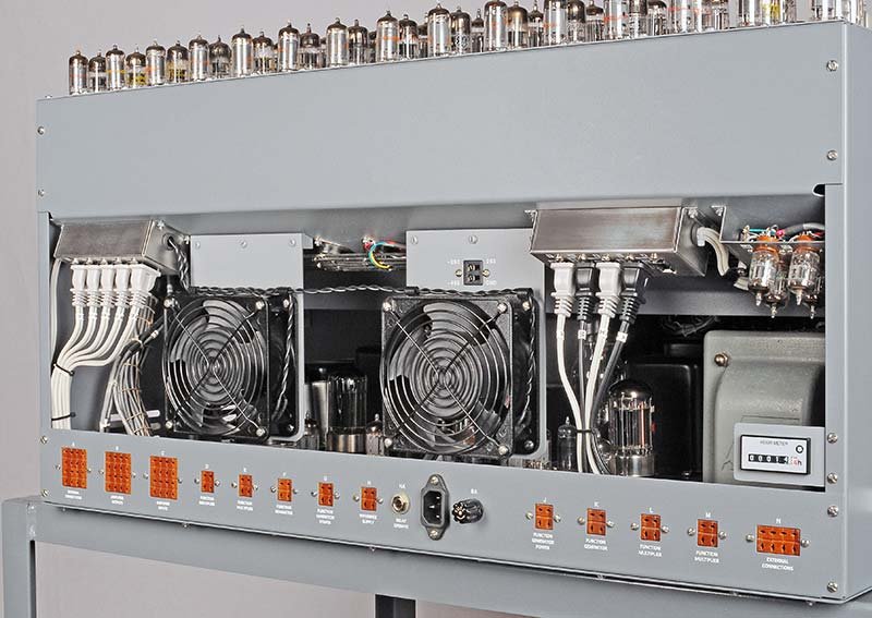
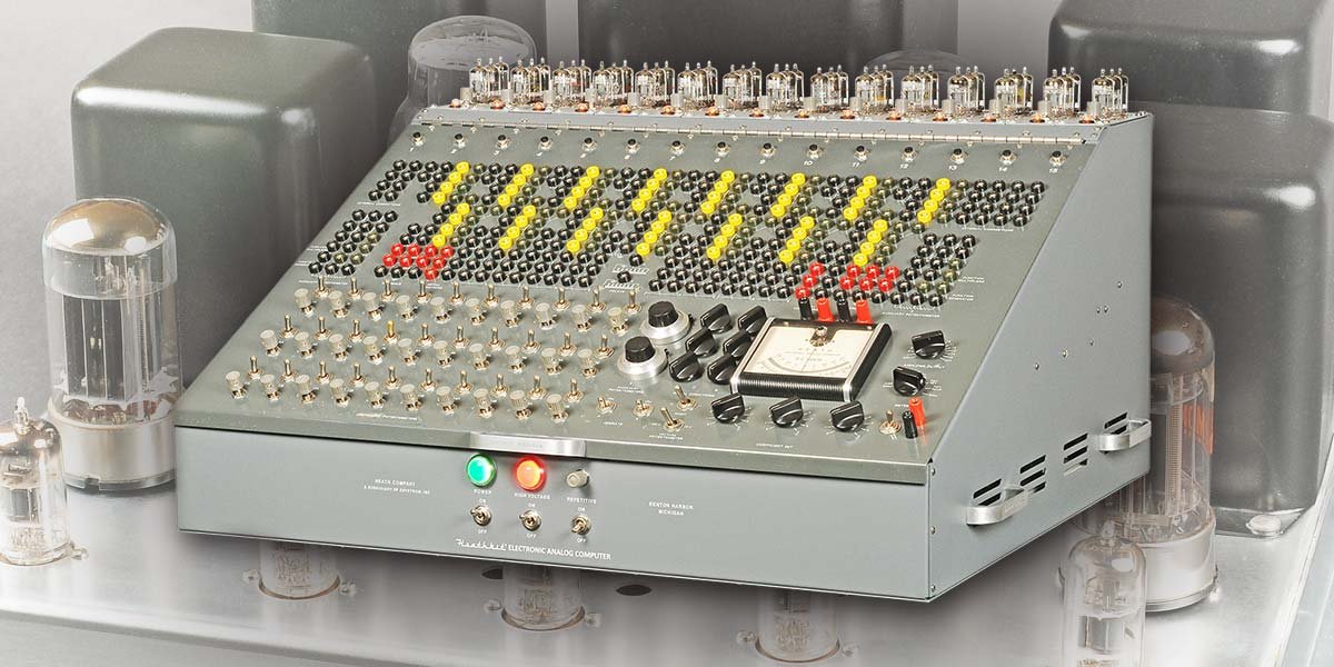
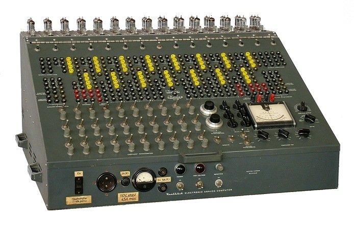 (The ES-400 in laboratory configuration. The 15 ES-201 operational amplifier modules are visible along the top row; the 364-jack patch panel dominates the front face.)
6.15 Next Steps
The demonstrations in this volume progress from a single-amplifier first-order system to a coupled nonlinear system using nine amplifiers. The remaining six ES-201 amplifiers are available for:
- Control-system demonstrations: closed-loop PID controller simulation (see Vol 7 when drafted)
- Electrical network simulation: RLC circuit transient response, transmission line approximations
- Thermal and fluid systems: heat conduction, laminar flow models
- Function generation using the ES-600: if the optional function generator is fitted, arbitrary periodic forcing functions become available, enabling resonance sweeps, random-noise forcing (via diode noise sources), and piecewise-linear approximations to nonlinear restoring forces
For the scaling methodology underlying all of these extensions, and for the general rules governing amplitude, time, and frequency scaling on the ES-400, see Vol 4. For the ES-201 amplifier’s open-loop gain, input-impedance model, and saturation behaviour that bound what is achievable without exceeding ±100 V, see Vol 2.
References
All values, component designations, and circuit topologies in this volume are derived from the following primary sources:
-
Heath Company. Heath Electronic Analog Computer Operational Manual. Heath Company, Benton Harbor, Michigan. (Original scanned PDF, rendered pages 1–28 reviewed for this volume.)
-
Goodsell, David. “Restoring the Heathkit ES-400 Computer.” Nuts & Volts Magazine, 2019. (Research Guide §1–§8 derived from this restoration article.)
-
Heath Company. ES-400 Research Guide. Compiled 2026. (Internal project reference document; Sections 7 and 8 consulted for all demo programs and scaling values.)
-
Johnson, C. L. Analog Computer Techniques. McGraw-Hill, 1956. (Referenced in ES-400 Operational Manual Appendix A.)
-
Warfield, J. N. Introduction to Electronic Analog Computers. Prentice-Hall, 1959. (Referenced in ES-400 Operational Manual Appendix A.)
Accuracy statement — All sub-assembly model numbers (ES-2, ES-50, ES-100, ES-151, ES-201, ES-505), tube types (12AX7, 6BQ7, 6BH6, NE-51), and voltage levels (±100 V signal, ±250 V plate supply, −450 V grid-bias) are verified against the Operational Manual and the 1956 Heath brochure (CHM accession 102646297). Coefficient-pot settings are derived from first principles and cross-checked against the Research Guide §8 where that section provides specific values (notably the 0.098 gravity-pot setting cited for free-fall). Where a value does not appear in the primary sources, it is explicitly labelled as “indicative” or “adjust empirically.”
Comments (0)