Heathkit ES-400 · Volume 5
Heathkit ES-400 — Volume 5 — Programming
Scaling, patching, and reading results — the complete operator workflow for turning differential equations into wired solutions on the ES-400
5.1 About this Volume
This volume covers the complete programming workflow for the Heath Electronic Analog Computer ES-400 (also designated the H-1). It assumes the reader has a functioning, calibrated machine — all fifteen ES-201 operational amplifiers balanced, the ES-2 amplifier supply delivering ±250 V and −450 V, and the ES-50 reference supply providing ±100 V. Readers who are still in acquisition, restoration, or bench-level troubleshooting should consult Vol 4 (Restoration & Alignment) first.
The ES-400 is a DC analog computer. Every signal treated in this volume is a slowly varying or static direct-current potential; “signal” never implies a radio-frequency carrier. The usable linear output range of each ES-201 module is ±100 V at up to 10 mA. The open-loop gain is approximately 50,000, so feedback configurations reach that ceiling very quickly — maintaining all variables comfortably inside ±100 V (ideally inside ±80 V with margin) is the central concern of scaling.
Note — Specific resistance and capacitance values quoted below (1 MΩ, 0.5 MΩ, 0.1 MΩ, 1 µF) are taken directly from the Heath Electronic Analog Computer Operational Manual (Heath Company, Benton Harbor, Michigan). The ES-400 is supplied with a resistor and capacitor kit; the operator selects and inserts appropriate components into the amplifier input and feedback jacks for each problem. Values not explicitly stated in that manual are noted as such.
Scope of this volume:
Table 1 — Scope of this volume:
| Section | Topic |
|---|---|
| 2 | The programming method — ODE to patch by successive integration |
| 3 | Magnitude scaling — choosing scale factors so variables stay within ±100 V |
| 4 | Time scaling — speeding up or slowing down the computer solution |
| 5 | Setting coefficients — potentiometers, resistor ratios, and the 10-turn auxiliaries |
| 6 | Reading results — meter, oscilloscope, and the repetitive mode |
| 7 | Full worked example end-to-end: the damped spring-mass-damper system |
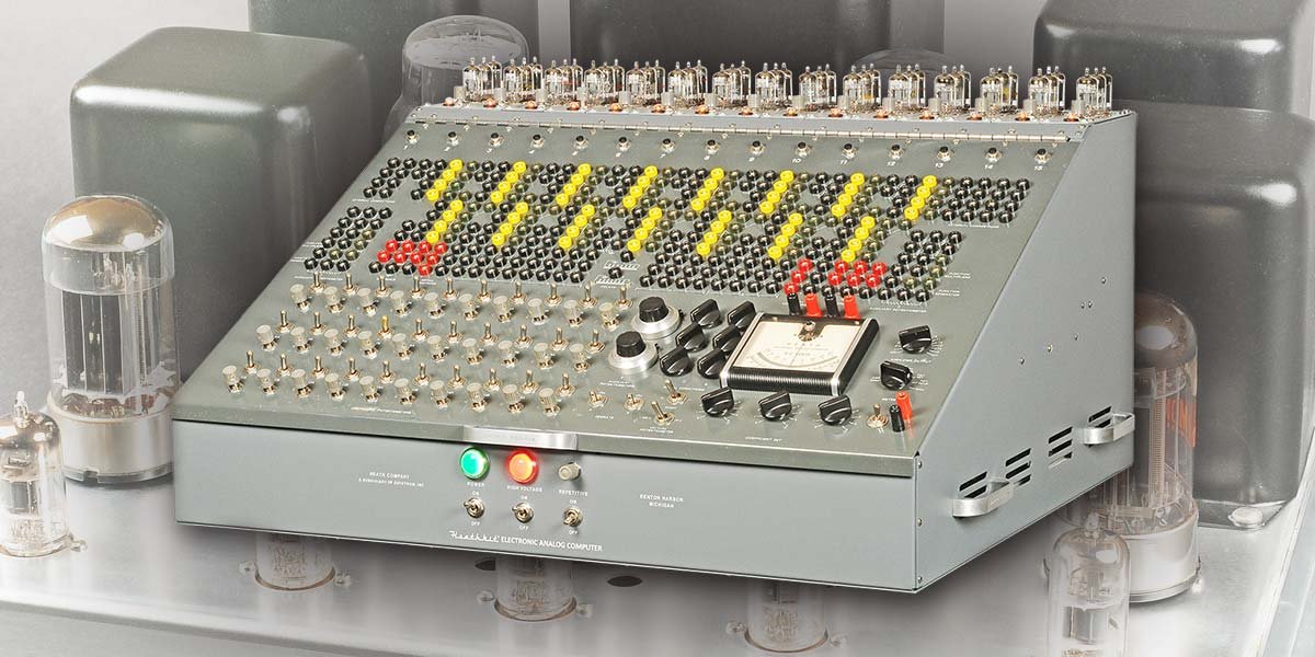
Figure 1 — The ES-400 in operation: a dense patch defining a multi-variable simulation. (Reference — courtesy Nuts & Volts / David Goodsell)
5.2 The Method — Turning an ODE into a Patch by Successive Integration
5.2.1 The Fundamental Insight
The ES-400 does not execute instructions or fetch data. When a problem is correctly patched, the machine is the differential equation — the electrical behavior of the wired network is mathematically isomorphic to the behavior of the physical system under study. Every variable in the problem corresponds to a DC voltage at a specific jack on the front panel, available at any moment simply by probing that jack with a voltmeter or oscilloscope.
The method rests on one key observation, stated explicitly in the Operational Manual:
Note — To solve a differential equation on an analog computer the procedure is generally as follows: (1) the initial conditions and the voltages are set up in the computer; (2) the computer is made operative and the voltages are formed to vary in the manner described by the given differential equation; (3) the machine is stopped and re-set to initial conditions, and is then ready for another run.
More specifically: any ordinary differential equation (ODE) of order n can be solved by a chain of n integrators, provided the highest-order derivative can be expressed as a function of lower-order derivatives and (possibly) the independent variable. This “feedback-around-integrators” or “successive-integration” technique is the universal programming strategy.
5.2.2 Step 1 — Write the ODE in Standard Form
Rearrange the problem equation so that the highest-order derivative stands alone on the left-hand side:
x''(t) = f(x', x, t)For an nth-order system, the right-hand side is a function of all derivatives up to order n−1. For the common second-order autonomous case (no explicit time dependence):
x'' = f(x', x)Example — forced spring-mass-damper:
Starting from Newton’s second law on a mass m with spring constant k, damping c, and external force F(t):
m·x'' + c·x' + k·x = F(t)Divide through by m:
x'' = (1/m)[F(t) − c·x' − k·x]This is the canonical form: the highest derivative equals a weighted sum of lower derivatives plus an input. Weighted sums are exactly what the ES-201 configured as a summer computes.
5.2.3 Step 2 — Assume the Highest Derivative Exists, Then Integrate Down
The programming trick: assume that the signal x'' is available at some summing point. Connect it to the first integrator; the integrator output is −x' (the minus sign arises from the inverting nature of the ES-201 in all configurations). Connect −x' to a second integrator to obtain +x. The signals x'', −x', and +x are now simultaneously available as voltages.
  x'' ──[INT-1: 1MΩ/1µF]──► −x' ──[INT-2: 1MΩ/1µF]──► +x
 (assumed at                                              │
  summing point)                                          │ feedback path
         ▲                                               │
         └──── summer computes f(−x', +x) ◄─────────────┘
The feedback path closes the loop: from the available signals −x' and +x, the right-hand side is computed and fed back to the summing point as x''. The loop is self-consistent — the circuit settles into the unique solution matching the initial conditions.
5.2.4 Step 3 — Draw the Block Diagram
Before a single patch cord is inserted, draw a complete block diagram on paper using standard analog-computer symbols. This is non-negotiable practice; errors caught on paper take seconds to fix, while errors found after patching may take hours to locate.
Standard Block Diagram Symbols:
─────────────────────────────────────────────────────────────────────
  Symbol           Meaning            ES-201 Configuration
─────────────────────────────────────────────────────────────────────
  ─[INT]─►         Integrator         Ri (input resistor), Cf (feedback cap)
  ─[SUM]─►         Summer/Inverter    Ri₁,Ri₂... (inputs), Rf (feedback res)
  ─[INV]─►         Inverter           Ri = Rf (unity gain summer, 1 input)
  ─(K)─►           Coefficient        Front-panel potentiometer 0–1
  ─(±Ref)          Reference voltage  ES-50: +100 V or −100 V DC
─────────────────────────────────────────────────────────────────────
The block diagram should show every amplifier used, the signal flowing into each input, the polarity at each output, and all feedback paths. Assign amplifier numbers (1–15, corresponding to the fifteen ES-201 modules) before patching.
5.2.5 Step 4 — Track Signs Through the Loop
The ES-201 is an inverting amplifier in every configuration:
- Integrator:
e_out = −(1/RC) ∫ e_in dt - Summer:
e_out = −(Rf/R₁)·e₁ − (Rf/R₂)·e₂ − ... - Inverter:
e_out = −e_in(when Ri = Rf)
A chain of two integrators introduces two inversions, resulting in a net positive sign. A chain of three introduces a net negative sign. Summers add further inversions. Tracking the sign at every node before patching prevents the most common programming error — a sign flip that converts a stable oscillation into a runaway exponential.
Sign-tracking table for the spring-mass-damper example:
Table 2 — Sign-tracking table for the spring-mass-damper example:
| Node | Expression | Sign | How obtained |
|---|---|---|---|
| A | x'' | + | Output of summer AMP-1 (inverted sum) |
| B | −x' | − | INT-1 output (integrates +x”) |
| C | +x | + | INT-2 output (integrates −x’) |
| Feedback | −(k/m)x − (c/m)(−x') + F/m | + | Summer computes, re-inverts |
Note — The Operational Manual states: “Linear mathematical operations are performed by using a high-gain D.C. amplifier.” The manual further notes that voltages may be added or subtracted simply by connecting inputs to the summing point with appropriate resistors, and that sign inversion is inherent in the amplifier. All sign-tracking must account for this inherent inversion.
5.2.6 Step 5 — Insert Components and Patch
With the block diagram verified on paper:
- Select resistors and capacitors from the ES-400 component kit for each amplifier.
- Insert input resistors into the numbered input jacks of each ES-201.
- Insert the feedback element (resistor for summer/inverter, capacitor for integrator) into the FEEDBACK jack.
- Run banana-plug patch cords between amplifier output jacks and the next amplifier’s input jacks as shown in the block diagram.
- Connect coefficient potentiometers in-line where scaling is required.
- Connect the appropriate IC supply output to each integrator’s initial-condition terminal.
Note — The Operational Manual specifies: “For satisfactory operation, capacitors used for integration must be of the highest quality. They should especially have very low leakage.” The manual recommends polystyrene or polyethylene type capacitors. The supplied capacitors are specifically selected for analog computer use.
5.2.7 The Mode Switches
The front panel provides two OPERATE RELAY switches (A and B) and access to the initial-condition (IC) supplies. Operating sequence:
┌─────────────────────────────────────────────────────────────────┐
│  Mode Sequence                                                  │
│                                                                 │
│  1. IC (Initial Condition) — relay connects IC supply to        │
│     integrator hold capacitors; outputs preset to x₀, x'₀     │
│                                                                 │
│  2. OPERATE — relays disconnect IC; integrators run freely;    │
│     the computation proceeds in real time                       │
│                                                                 │
│  3. (Manual or repetitive reset back to IC for next run)       │
└─────────────────────────────────────────────────────────────────┘
The Operational Manual states: “In order to avoid bias, it is necessary that the relay be connected to the input of the amplifier and not to the output.” The relay contacts appear explicitly in the manual’s circuit diagrams (Figure 5, page 5 of the Operational Manual).
┌─────────────────────────────────────────────────────────────────────────────┐
│                    ES-400 PROGRAMMING FLOW                                  │
│                                                                             │
│  Physical Problem                                                           │
│        │                                                                    │
│        ▼                                                                    │
│  Write ODE in standard form: x'' = f(x', x, t)                             │
│        │                                                                    │
│        ▼                                                                    │
│  Apply magnitude scaling: choose α such that |α·x| ≤ 80 V                  │
│        │                                                                    │
│        ▼                                                                    │
│  Apply time scaling: choose β such that solution completes in              │
│  observable window (0.1 s – several seconds)                                │
│        │                                                                    │
│        ▼                                                                    │
│  Draw block diagram — label every node, sign, amplifier number             │
│        │                                                                    │
│        ▼                                                                    │
│  Select component values (R, C, pot settings)                               │
│        │                                                                    │
│        ▼                                                                    │
│  Insert components → run patch cords → set IC supplies                      │
│        │                                                                    │
│        ▼                                                                    │
│  Balance check: short all inputs, verify each amp output = 0 V             │
│        │                                                                    │
│        ▼                                                                    │
│  IC mode → verify initial conditions at key jacks                           │
│        │                                                                    │
│        ▼                                                                    │
│  OPERATE → observe on meter / oscilloscope                                  │
│        │                                                                    │
│        ▼                                                                    │
│  Adjust pots → parameter study → refine scaling if needed                   │
└─────────────────────────────────────────────────────────────────────────────┘
Figure 2 — ES-400 programming workflow from physical problem to observed solution.
5.3 Magnitude Scaling
5.3.1 Why Scaling Is Necessary
The ES-201 operates linearly only within its ±100 V output range. If a physical variable — say, a displacement measured in meters — were mapped directly to volts without scaling, the solution would be meaningless: a 1-meter displacement would correspond to 1 V and be difficult to observe, while a 150-meter trajectory would saturate the amplifiers at ±100 V and trigger the NE-51 overload indicators. Both extremes are unacceptable.
Magnitude scaling defines a relationship between each physical variable and its corresponding machine voltage:
e_variable = α · x_physicalwhere α (volts per physical unit) is chosen so that the maximum expected value of |x_physical| maps to no more than roughly 80–90 V — leaving headroom before the ±100 V rail.
Danger — Operating the ES-201 with its output at or beyond ±100 V saturates the output stage. The NE-51 neon indicator on the front of each module lights to signal this condition. In saturation the amplifier is no longer computing correctly, and the feedback loop behavior may be erratic. Any NE-51 illumination during a run indicates the scaling must be revised.
5.3.2 Choosing Scale Factors
Step 1 — Estimate the maximum of each variable. From the physics of the problem, or from a rough hand calculation, determine the maximum expected magnitude of each variable and its significant derivatives. For example, in a free-fall problem with a maximum drop height of 100 m:
|x|_max ≈ 100 m
|x'|_max ≈ √(2g·100) ≈ 44 m/s
|x''|_max = g ≈ 9.8 m/s²
Step 2 — Choose voltage scale factors. Assign scale factors α_x, α_v, α_a (for position, velocity, acceleration respectively) such that:
α_x · 100 m ≤ 80 V   →   α_x ≤ 0.8 V/m   →   choose α_x = 0.5 V/m
α_v · 44 m/s ≤ 80 V  →   α_v ≤ 1.82 V·s/m →   choose α_v = 1.5 V·s/m
α_a · 9.8 m/s² ≤ 80V →   α_a ≤ 8.2 V·s²/m →  choose α_a = 5.0 V·s²/m
Step 3 — Rewrite the equation in machine variables. Let u = α_x · x, v = α_v · x', w = α_a · x''. Substitute into the ODE and collect terms to find the scaled equation that the machine will solve. The scale factors introduce additional constant multipliers that may be absorbed into resistor ratios or pot settings.
5.3.3 Machine Variables and Dimensional Consistency
The machine equation must be dimensionally consistent in volts. The integration operation performed by the ES-201 with a 1 MΩ input resistor and 1 µF feedback capacitor has a time constant of:
τ = R·C = 1×10⁶ Ω × 1×10⁻⁶ F = 1 secondso its output is:
e_out = −(1/τ) ∫ e_in dt = −∫ e_in dt [with τ = 1 s, both voltages in volts, time in seconds]This is exactly the relationship needed for problems where the natural time unit is seconds. For faster or slower problems, time scaling (Section 4) adjusts the effective τ.
5.3.4 Scaling Table for the Free-Fall Example
Table 3 — Scaling Table for the Free-Fall Example
| Variable | Physical Quantity | Max Value | Scale Factor | Max Machine Voltage |
|---|---|---|---|---|
u | Position x (m) | 100 m | 0.5 V/m | 50 V |
v | Velocity x’ (m/s) | 44 m/s | 1.5 V·s/m | 66 V |
w | Acceleration x” (m/s²) | 9.8 m/s² | 5.0 V·s²/m | 49 V |
r | Reference (constant) | 100 V | — | 100 V (ES-50 rail) |
All values comfortably within ±80 V — adequate margin before saturation.
5.3.5 Cascade Scaling: Tracking Units Through Integrators
Each integrator introduces a factor of 1/τ (where τ is in seconds) and changes the dimension by one factor of time. When the machine time equals the problem time (β = 1, see Section 4), this factor is unity. When time scaling is applied, the effective time constant changes and these factors must be recomputed.
Physical:   x'' ──[∫ dt]──► x' ──[∫ dt]──► x
Machine:    w   ──[1/τ]───► v  ──[1/τ]───► u

Constraint: v/τ = u   implies   α_v · x' / τ = α_x · x
            With τ = 1s: α_v = α_x  (if x' and x have the same scale factor)
            In general: α_v = α_x · τ
This constraint links the scale factors of adjacent variables in an integrator chain. It does not have to be satisfied exactly — a pot can absorb any residual ratio — but violating it significantly forces pot settings to extreme values (near 0 or near 1) that are difficult to read accurately.
5.4 Time Scaling
5.4.1 Motivation
A physical problem may evolve over a time span that is either too fast or too slow to observe conveniently:
- A missile trajectory might unfold in 30 seconds — fine for the oscilloscope, but each run wastes operator time.
- A thermal transient in a building might take 8 hours — impossible to run in real time.
- A nuclear reactor transient might develop in milliseconds — far too fast for the oscilloscope to display at slow sweep.
Time scaling compresses or expands the computer time relative to the problem time by a factor β:
t_computer = β · t_problemWhen β > 1, the computer runs faster than real time (slow-motion display of a fast physical process). When β < 1, the computer runs slower than real time.
5.4.2 Effect on Integration Time Constants
The standard 1 MΩ / 1 µF integrator has τ = 1 s. To achieve a time scale factor β, the effective integration time constant must be changed to τ_eff = τ/β. This is accomplished by changing either the resistor or the capacitor value.
The Operational Manual provides the standard component values available in the ES-400 kit:
Table 4 — The Operational Manual provides the standard component values available in the ES-400 kit
| Resistor (MΩ) | Capacitor (µF) | τ = RC (seconds) | Time scale factor β (relative to τ=1s reference) |
|---|---|---|---|
| 1.0 | 1.0 | 1.0 | 1× (real time, if problem time unit = 1 s) |
| 0.5 | 1.0 | 0.5 | 2× (computer runs twice as fast) |
| 0.1 | 1.0 | 0.1 | 10× |
| 1.0 | 0.5 | 0.5 | 2× |
| 0.1 | 0.1 | 0.01 | 100× |
Note — The resistor values available in the ES-400 component kit are 0.1 MΩ, 0.5 MΩ, and 1 MΩ per the Operational Manual. Capacitor values are similarly limited to those supplied. Intermediate time-scale factors can be achieved by adjusting pot settings in the signal path, though this changes gains as well and requires recomputing scale factors.
5.4.3 Repetitive Mode and the ES-505 Oscillator
The ES-505 Repetitive Oscillator (0.6–6 Hz) drives the OPERATE RELAYs at a selectable repetition rate, automatically cycling the machine between IC and OPERATE modes. This allows the computation to repeat continuously, creating a steady display on an oscilloscope. The operator sets up the oscilloscope’s horizontal sweep to match the ES-505 frequency so that successive traces overlap.
ES-505 Oscillator (0.6–6 Hz)
       │
       ▼
  OPERATE RELAY A ──── controls IC/OPERATE switching of integrators
  OPERATE RELAY B ──── available for additional mode control
       │
       ▼
  At each cycle:
    IC phase:      integrator capacitors charged to initial conditions
    OPERATE phase: free computation proceeds for (1/f) seconds
    IC phase:      reset for next cycle
The Operational Manual states: “For the falling body problem a time constant of 1 is suitable. In practice, this means no need for the repetitive oscillator.” For problems with short solution times, however, the repetitive oscillator is essential for maintaining a stable oscilloscope display.
Note — When using the repetitive oscillator for oscilloscope display, it is convenient to connected the Y output of the computer to the vertical (Y) input of the oscilloscope, and to use the oscilloscope’s own time base for the horizontal axis. Alternatively, an independent variable (such as time itself, derived from integrating a constant reference voltage) can drive the oscilloscope’s horizontal input in XY mode.
5.4.4 Time-Scaling Worked Calculation
Problem: The natural period of a spring-mass system is T = 2π√(m/k) = 2 seconds. The computation would complete in roughly one period. A 2-second run on the oscilloscope is acceptable. No time scaling is required; β = 1, and 1 MΩ / 1 µF components are used throughout.
Modified problem: The spring is stiff — T = 0.02 seconds. At β = 1, the transient decays before the oscilloscope can capture it on a slow sweep. Choose β = 100 (speed up by ×100):
τ_eff = 1 s / 100 = 0.01 s
Use 0.1 MΩ input resistors and 0.1 µF capacitors throughout.
With β = 100, a 0.02-second physical oscillation appears as a 2-second computer oscillation — easily captured and displayed.
5.5 Setting Coefficients
5.5.1 The Coefficient Potentiometers
The ES-400 front panel provides thirty (30) coefficient potentiometers plus two (2) auxiliary 10-turn potentiometers. Each standard pot is a single-turn, wire-wound unit with a dial calibrated 0–10 on its face; the actual attenuation is 0–1 (maximum clockwise = full input voltage through). The 10-turn auxiliary pots provide finer resolution for coefficients that must be set accurately.
Coefficient pot output = (dial reading / 10) × input voltageFor example, with the pot set to 3.7 and a +100 V reference at its input:
e_out = (3.7/10) × 100 V = 37 VThe Operational Manual describes the coefficient-setting procedure:
- Turn the METER switch to the AMPLIFIER OUTPUT position.
- With only the coefficient pot supply connected, adjust the pot dial until the meter reads the desired voltage (not the desired dial number, since wire-wound pots may not be perfectly linear).
- With the meter as a reference standard, the pot can be set to any fraction of the input voltage within the accuracy of the meter.
- The INVERT toggle switch on the meter section inverts the polarity, allowing verification of negative voltages.
Note — The Operational Manual specifies: “At times it may be desirable to null the output of an amplifier. The voltage is applied to the input of the coefficient potentiometer which was previously set at ‘amp zero’ position. Press the invert toggle switch to the ’−’ position.” This allows the pot to serve as a fine-trim null adjustment when setting up an initial condition.
5.5.2 Setting Coefficients from Scaled Equations
After magnitude and time scaling, the ODE coefficients become dimensionless machine constants. These constants are realized by combinations of:
- Resistor ratios — the gain of a summer in the input-resistor configuration is
Rf/Ri(before the sign inversion). Standard resistors in the kit give ratios of 0.1, 0.5, 1, 2, 5, and 10. - Pot settings — any coefficient between 0 and 1 (after resistor gain is applied). The pot setting is
K = coefficient / resistor_gain. - Combined (resistor × pot) — for coefficients between 0 and 10, use a 1 MΩ feedback resistor with a 0.1 MΩ input resistor (gain = 10) and set the pot to
K = coefficient / 10.
Coefficient allocation table:
Table 5 — Coefficient allocation table:
| Coefficient Range | Resistor Configuration | Pot Setting K |
|---|---|---|
| 0 to 1.0 | Ri = Rf = 1 MΩ (gain = 1) | K = coefficient |
| 0 to 2.0 | Ri = 0.5 MΩ, Rf = 1 MΩ (gain = 2) | K = coefficient / 2 |
| 0 to 5.0 | Ri = 0.2 MΩ (not in kit) or two 0.1 MΩ in series | K = coefficient / 5 |
| 0 to 10.0 | Ri = 0.1 MΩ, Rf = 1 MΩ (gain = 10) | K = coefficient / 10 |
| Fixed integer | Ri ratio alone (no pot) | — |
Note — The Operational Manual notes: “The coefficient potentiometers are set with the amplifier output switch in any position and the meter switch in ‘POT SET’ mode.” In POT SET mode, the meter reads the output of whichever pot is being adjusted, scaled by the input reference voltage.
5.5.3 Auxiliary 10-Turn Potentiometers
The two 10-turn pots on the front panel are reserved for coefficients that must be set with high precision — typically the natural frequency ω or damping ratio ζ in a problem being studied parametrically. A standard single-turn pot has perhaps 2% setting accuracy; the 10-turn units provide roughly 0.2% resolution. This is important when searching for critical-damping conditions or when the problem coefficient is known analytically and must be matched exactly.
5.5.4 Initial Condition Supplies (ES-100)
The three ES-100 Initial Condition Power Supply modules each provide two isolated 100 V floating supplies. These feed the IC terminals of the integrators when the relay is in IC mode, presetting each integrator’s output to a specific voltage representing the initial value of that variable.
Table 6 — Initial Condition Supplies (ES-100)
| IC Supply | Typical Assignment | Accessible From |
|---|---|---|
| IC-1 (positive) | x₀ (initial position) | Front panel IC jacks |
| IC-1 (negative) | −x₀ | Front panel IC jacks |
| IC-2 (positive) | v₀ (initial velocity) | Front panel IC jacks |
| IC-2 (negative) | −v₀ | Front panel IC jacks |
| IC-3 (positive/negative) | Higher-order or additional variables | Front panel IC jacks |
The IC voltage is set by the IC supply’s front-panel adjustment, monitored with the panel meter in AMPLIFIER OUTPUT mode.
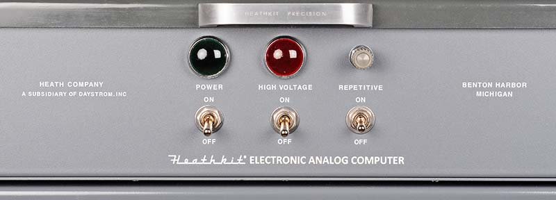
Figure 3 — Power panel on the fully restored ES-400. The green lamp indicates mains power, red lamp indicates high voltage (±250 V / −450 V on the ES-2), and white lamp indicates the ES-505 repetitive oscillator is running. (Reference — courtesy Nuts & Volts / David Goodsell)
5.6 Reading Results
5.6.1 The Panel Meter
The ES-400 includes a DC milliammeter on the front panel (converted to read voltage via a series resistor network). The METER switch selects among:
┌──────────────────────────────────────────────────────────────────┐
│  METER SWITCH POSITIONS                                          │
│                                                                  │
│  AMP ZERO          — amplifier balance (zero) mode; reads the   │
│                       selected amplifier output for nulling      │
│                                                                  │
│  POT SET           — reads the output of the potentiometer       │
│                       being adjusted (coefficient setting)       │
│                                                                  │
│  POT READ          — reads the pot output with reference         │
│                       connected; verifies coefficient value      │
│                                                                  │
│  NULL              — output nulling mode; used with the          │
│                       AMPLIFIER OUTPUT jack for zero-checking    │
└──────────────────────────────────────────────────────────────────┘
The INVERT switch on the meter section applies a sign flip to allow reading of negative voltages on the upscale meter movement. The Operational Manual states: “At times it may be desirable to null the output of an amplifier. The voltage is applied to the input of the coefficient potentiometer which was previously set at zero. Press the invert toggle switch to the ’−’ position. Turn the pot until the meter reads zero.”
The meter is adequate for setting up initial conditions and checking static pot values, but it is too slow and too coarse to observe the dynamic behavior of a running computation. That function belongs to the oscilloscope.
5.6.2 Oscilloscope Connection
The oscilloscope is the ES-400’s primary dynamic display instrument. Any amplifier output jack is a low-impedance source (the ES-201 drives ±100 V at up to 10 mA) capable of driving an oscilloscope input with negligible loading, provided the oscilloscope input impedance is 1 MΩ or higher — standard for any instrument of the era or later.
Time-domain display (Y-vs-t): Connect one amplifier output to the oscilloscope’s vertical (Y) input. Set the oscilloscope’s horizontal sweep to match the expected solution duration. If the repetitive oscillator is in use, trigger the oscilloscope from the ES-505 output for a stable, repeating trace.
Phase-plane display (Y-vs-X): Connect one variable (e.g., displacement x) to the oscilloscope Y input and another variable (e.g., velocity x') to the X input. Select XY mode on the oscilloscope. The result is a phase-plane trajectory — the curve traced by the state vector (x, x') over time. Phase-plane displays reveal damping behavior, limit cycles, and equilibrium points at a glance.
Lissajous figures: Connect two independent oscillator outputs to X and Y inputs. If the frequency ratio is a simple fraction, a stable geometric figure appears. This technique historically served to compare and calibrate frequency standards.
5.6.3 Repetitive Display Setup
┌────────────────────────────────────────────────────────────────┐
│  REPETITIVE DISPLAY PROCEDURE                                  │
│                                                                │
│  1. Set ES-505 repetition rate f (0.6–6 Hz).                  │
│  2. Ensure REPETITIVE switch on power panel is ON.            │
│  3. Connect oscilloscope vertical input to desired output.     │
│  4. Set oscilloscope sweep to 1/f seconds full-scale.         │
│  5. Trigger oscilloscope from ES-505 output jack OR use       │
│     oscilloscope's own internal trigger on the signal.        │
│  6. Overlapping traces confirm solution is reproducible.      │
│  7. Adjust pot settings in real time; traces update           │
│     immediately with no re-patching required.                 │
└────────────────────────────────────────────────────────────────┘
The Operational Manual’s Figure 20 (page 16 of the manual) shows actual oscilloscope recordings from the ES-400 of a free-fall trajectory — position vs. time — demonstrating that the machine produces the theoretically expected parabolic curve.
5.6.4 Reading Accuracy and Overload Detection
The NE-51 neon lamp on the face of each ES-201 module illuminates when the amplifier output exceeds its linear range. During a run, the operator should observe all fifteen NE-51 indicators. Any lamp that glows indicates overload on that amplifier — the corresponding variable’s scale factor must be reduced (or the time scale adjusted) before results from that amplifier can be trusted.
Table 7 — Reading Accuracy and Overload Detection
| Indicator | Location | Interpretation |
|---|---|---|
| GREEN lamp (POWER ON) | Power panel | Mains applied to the ES-401 transformer |
| RED lamp (HIGH VOLTAGE ON) | Power panel | ES-2 ±250 V / −450 V rails live |
| WHITE lamp (REPETITIVE ON) | Power panel | ES-505 oscillator running |
| NE-51 neon (×15) | Each ES-201 module | Overload on that amplifier |
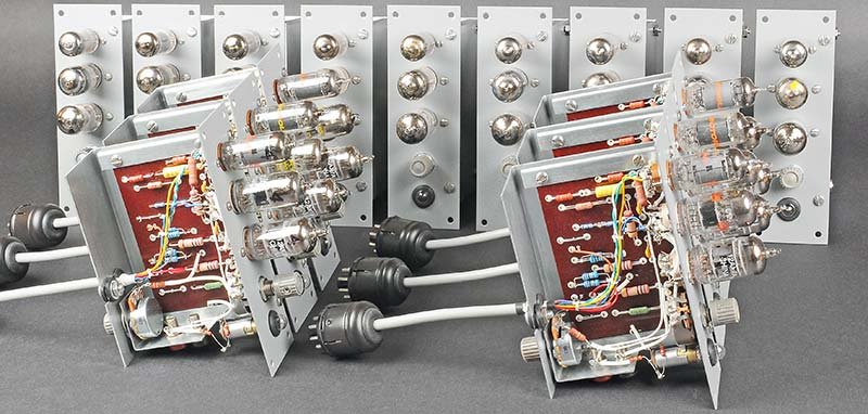
Figure 4 — Fifteen ES-201 modules after restoration. Each carries three vacuum tubes (12AX7 input stage, 6BQ7 intermediate, 6BH6 output pentode) and the NE-51 overload indicator. These modules slide into the interior of the ES-400 cabinet and connect to the front panel harness via their rear multi-pin connectors. (Reference — courtesy Nuts & Volts / David Goodsell)
5.7 Full Worked Example — Damped Spring-Mass-Damper System
5.7.1 Problem Statement
Model the step response of a single-degree-of-freedom linear mechanical system: a mass m on a spring (stiffness k) with a viscous damper (damping coefficient c), subject to a step forcing function F₀ at t = 0.
Equation of motion:
m·x'' + c·x' + k·x = F₀·u(t)where u(t) is the unit step function (zero before t = 0, unity for t > 0, implemented as the ES-50 +100 V reference switched via a pot).
Design goal: Demonstrate the transition from underdamped to critically damped to overdamped response by turning a single front-panel pot.
Specific numerical parameters (chosen to give convenient machine values):
m = 1 kg         (normalized — divides out)
k = 100 N/m      (natural frequency ω_n = √(k/m) = 10 rad/s, T_n ≈ 0.63 s)
c = variable     (damping ratio ζ = c / (2·√(k·m)) = c / 20)
F₀ = 50 N        (step amplitude)
Physical maxima (estimated):
x_max ≈ F₀/k = 50/100 = 0.5 m  (static deflection under full load)
x'_max ≈ ω_n · x_max ≈ 10 × 0.5 = 5 m/s
x''_max ≈ F₀/m = 50 m/s²   (initial acceleration at t=0⁺)
Initial conditions:
x(0) = 0   (mass at rest at equilibrium)
x'(0) = 0  (zero initial velocity)
5.7.2 Step 1 — Rearrange into Standard Form
x'' = (1/m)[F₀ − c·x' − k·x]
   = F₀ − (c/m)·x' − (k/m)·x
   = 50 − c·x' − 100·x          (with m=1)
5.7.3 Step 2 — Magnitude Scaling
Choose scale factors based on the physical maxima:
u = α_x · x,    α_x = 100 V / 0.5 m = 200 V/m  → too large, use α_x = 100 V/m
v = α_v · x',   α_v = 100 V / 5 m/s = 20 V·s/m
w = α_a · x'',  α_a = 100 V / 50 m/s² = 2 V·s²/m
Check: u_max = 100×0.5 = 50 V, v_max = 20×5 = 100 V (borderline — reduce to α_v = 15), w_max = 2×50 = 100 V (borderline — reduce to α_a = 1.5). After adjustment:
Table 8 — Check: umax = 100×0.5 = 50 V, vmax = 20×5 = 100 V (borderline — reduce to αv = 15), wmax = 2×50 = 100 V (borderline — reduce to αa = 1.5). After adjustment
| Machine Variable | Physical Variable | Scale Factor | Peak Machine Voltage |
|---|---|---|---|
u (displacement) | x (m) | α_x = 100 V/m | 50 V |
v (velocity) | x' (m/s) | α_v = 15 V·s/m | 75 V |
w (acceleration) | x'' (m/s²) | α_a = 1.5 V·s²/m | 75 V |
5.7.4 Step 3 — Time Scaling
With ω_n = 10 rad/s, the natural period is T_n ≈ 0.63 seconds. A critically damped response decays to near-zero in roughly 3T_n ≈ 2 seconds. This is comfortable for real-time oscilloscope display. Choose β = 1 (no time scaling); use 1 MΩ resistors and 1 µF capacitors throughout.
5.7.5 Step 4 — Write the Scaled Machine Equation
Substitute x = u/α_x, x' = v/α_v, x'' = w/α_a into the physical ODE:
(w/α_a) = F₀ − (c/m)·(v/α_v) − (k/m)·(u/α_x)
w = α_a · [F₀ − (c)·(v/α_v) − (100)·(u/α_x)]
w = α_a·F₀ − α_a·c·(v/α_v) − α_a·100·(u/α_x)
w = 1.5×50 − 1.5·c·(v/15) − 1.5×100·(u/100)
w = 75 − (c/10)·v − 1.5·u
Machine equation (all voltages):
w = 75·(1 V/V) − (c/10)·v − 1.5·uThis is the equation the summer (AMP-1) must implement. Coefficients:
A₁ = coefficient on reference (+100 V): 75/100 = 0.75  → pot P1 set to 7.5 (dial)
A₂ = coefficient on v: c/10 (variable damping pot P2)
A₃ = coefficient on u: 1.5  → use 0.5 MΩ input, 1 MΩ feedback → gain = 2; pot P3 = 0.75
Note — The summer AMP-1 inverts its output: its output is
−w. The integrators will negate again as needed — sign tracking is essential here.
5.7.6 Step 5 — Block Diagram
                        ┌──────────────────────────────────────────┐
                        │                                          │
+100V ref ──[P1=0.75]──►┤                                          │
                        │  AMP-1 (SUMMER)           ┌─────────────┴────┐
      −v ──[P2=c/10]───►│  Ri=1MΩ, Rf=1MΩ         │                  │
                        │  Output: −w              │  AMP-2 (INT-1)   │
      −u ──[P3=0.75]───►│  = −75 + (c/10)v + 1.5u  │  Ri=1MΩ, Cf=1µF │
                        └──────────────────────────►│  Output: +v      │
                                                    │  = −∫(−w)dt     │
                                                    │  = +∫w dt        │
                                                    └────────┬─────────┘
                                                             │
                                                    ┌────────▼─────────┐
                                                    │  AMP-3 (INT-2)   │
                                                    │  Ri=1MΩ, Cf=1µF │
                                                    │  Output: −u      │
                                                    │  = −∫v dt        │
                                                    └────────┬─────────┘
                                                             │
                                           (−u)─────────────┘
                                           feedback to AMP-1 (−u input → AMP-1 inverts → +1.5u in w)
Complete signal list:
Table 9 — Complete signal list:
| Node | Voltage | Physical Meaning |
|---|---|---|
| AMP-1 output | −w | Scaled acceleration (negated) |
| AMP-2 output | +v | Scaled velocity |
| AMP-3 output | −u | Scaled displacement (negated) |
| P1 wiper | +75 V | Scaled forcing function |
| P2 wiper | (c/10)·v | Damping term input to AMP-1 |
5.7.7 Step 6 — Component Selection
Table 10 — Step 6 — Component Selection
| Amplifier | Role | Input Resistors | Feedback Element |
|---|---|---|---|
| AMP-1 | Summer | 3 × 1 MΩ (one per input) | 1 MΩ (resistor) |
| AMP-2 | INT-1 | 1 MΩ | 1 µF (capacitor) |
| AMP-3 | INT-2 | 1 MΩ | 1 µF (capacitor) |
Total ES-201 modules used: 3 of 15.
5.7.8 Step 7 — Patch List
The following patch cords are required. Colors follow the convention used in the Operational Manual (Figure 13/14, page 12): black for ground returns, yellow or green for signal paths, red for reference connections.
Table 11 — Step 7 — Patch List
| From Jack | To Jack | Color | Function |
|---|---|---|---|
| ES-50 +100 V | P1 input jack | Red | Forcing function reference |
| P1 wiper | AMP-1 input 1 | Yellow | Scaled F₀ input |
| AMP-2 output (+v) | P2 input jack | Green | Velocity feedback |
| P2 wiper | AMP-1 input 2 | Green | Damping term |
| AMP-3 output (−u) | AMP-1 input 3 | Yellow | Displacement feedback |
| AMP-1 output (−w) | AMP-2 input | Yellow | Acceleration to INT-1 |
| AMP-2 output (+v) | AMP-3 input | Green | Velocity to INT-2 |
| IC-1 (+) | AMP-2 IC terminal | White | x’(0) = 0 V |
| IC-2 (+) | AMP-3 IC terminal | White | x(0) = 0 V |
| AMP-3 output (−u) | Oscilloscope CH1 | — | Displacement (inverted sign — note on chart) |
| AMP-2 output (+v) | Oscilloscope CH2 | — | Velocity |
Total patch cords: 11 plus oscilloscope connections. (The Operational Manual’s bouncing ball demonstration uses 35 cords across 9 amplifiers, to give a sense of the scale of more complex problems.)
5.7.9 Step 8 — Pre-Run Checks
Balance check:
- Remove all input connections from each amplifier.
- Short the summing junction (input) of each ES-201 to signal ground.
- Verify that the METER (AMPLIFIER OUTPUT mode) reads zero at each amplifier’s output.
- If not, adjust the BALANCE pot for that amplifier (see Vol 4 for the balancing procedure).
IC verification:
- Set OPERATE RELAYs to IC mode.
- Set P1, P2, P3 to zero (pots fully counterclockwise).
- Verify that AMP-2 output = 0 V (x’₀ = 0) using the meter.
- Verify that AMP-3 output = 0 V (x₀ = 0) using the meter.
- Set P1 to 7.5 (dial), P3 to 7.5 (dial), P2 to a starting value for ζ = 0.1 (underdamped):
P2 = c/10 = (2ζω_n·m)/10 = (2×0.1×10×1)/10 = 0.2→ dial setting 2.0.
Component verification:
The Operational Manual reminds the operator: “It is now necessary to check that there is a relay in the system. The relay will generally prevent current flow through the feedback impedance unless the relay is in the correct position.” Confirm IC/OPERATE relay behavior before running.
5.7.10 Step 9 — Run and Observe
- Ensure POWER ON and HIGH VOLTAGE ON. Allow 30 minutes warm-up for tube stabilization.
- With REPETITIVE ON and ES-505 set to ~1 Hz, the computation cycles automatically.
- Observe AMP-3 output on oscilloscope (displacement vs. time).
- Observe AMP-2 output (velocity vs. time) on second oscilloscope channel.
- For phase-plane display: connect AMP-3 → oscilloscope X, AMP-2 → oscilloscope Y, select XY mode.
Expected waveforms:
Table 12 — Expected waveforms:
| P2 Setting (ζ) | AMP-3 Output | Oscilloscope Appearance |
|---|---|---|
| 2.0 (ζ ≈ 0.1) | Underdamped — decaying sinusoid, overshoots | Spiral converging to equilibrium (phase plane) |
| 10.0 (ζ = 0.5) | Underdamped — fewer oscillations | Tighter spiral |
| 20.0 (ζ = 1.0) | Critically damped — monotonic approach, fastest | Phase-plane: single curve to equilibrium |
| 40.0 (ζ = 2.0) | Overdamped — slow exponential approach | Phase-plane: broader, slower curve |
5.7.11 Step 10 — Parameter Study
The ES-400’s greatest advantage over digital simulation is the ability to explore parameter space in real time. With the problem patched and running:
- Turn P2 slowly from 2.0 to 40.0 — watch the oscilloscope trace transition continuously through all damping regimes.
- Turn P1 (forcing amplitude) to change the step size — the steady-state deflection and transient peaks scale proportionally.
- Change P3 to explore stiffness variation — increase the spring constant (higher P3 within its gain range) while maintaining the same damping, watching the frequency increase while the envelope changes.
None of these adjustments require re-patching. They are instantaneous and continuous — a fundamental capability of analog computation that no digital simulation of the era could match.
Note — The Operational Manual summarizes this capability: “Ordinarily the value of RC is the same as the coefficient for the integrating capacitors. Repetitive operation is used when the problem allows a cathode ray oscilloscope. This may be done in a relatively short time. For the falling body problem a time constant of 1 is suitable.” This underscores that even for complex demonstrations, the machine is operated interactively, with the operator adjusting parameters and immediately observing the effect on the displayed waveform.
5.7.12 Signal-Flow Diagram for the Worked Example
+100V ──[P1: 0.75]──────────────────────────────────┐
                                                    │
                           ┌────────────────────────▼────────────────┐
                           │          AMP-1 (SUMMER)                  │
           ┌──[P2: c/10]───┤  −w = −[0.75×100 − (c/10)v − 1.5u]    │
           │               │  Ri=1MΩ×3, Rf=1MΩ                       │
           │   ┌──[P3:0.75]┤                                          │
           │   │           └──────────────────────┬───────────────────┘
           │   │                                  │ −w (scaled accel, negated)
           │   │(−u) from AMP-3                   │
           │   │                                  ▼
           │   │                    ┌──────────────────────────────┐
           │   │                    │  AMP-2 (INT-1)               │
           │   │                    │  Ri=1MΩ, Cf=1µF              │
           │   │                    │  +v = −∫(−w)dt = +∫w dt     │
           │   │             ┌──────┤  (velocity, correct sign)    │
           │   └─────────────┘      └──────────────────────────────┘
           │   (+v) feedback                      │ +v
           └───────────────────────────────────   │
                                                  ▼
                                    ┌──────────────────────────────┐
                                    │  AMP-3 (INT-2)               │
                                    │  Ri=1MΩ, Cf=1µF              │
                                    │  −u = −∫v dt                 │
                                    │  (displacement, negated)     │
                                    └──────────────┬───────────────┘
                                                   │ −u
                            ┌──────────────────────┘
                            │ (fed back to P3 input and AMP-1)
                            ▼
                      Oscilloscope
                      (negate reading to get +u = displacement)
Figure 5 — Complete signal-flow diagram for the spring-mass-damper example. Three ES-201 amplifiers implement the second-order ODE; three potentiometers set the coefficients; two IC supplies preset initial conditions to zero.
5.8 Reference Tables
5.8.1 ES-400 Computing Element Summary
Table 13 — ES-400 Computing Element Summary
| Element | ES-201 Config | Input | Feedback | Transfer Function | Sign |
|---|---|---|---|---|---|
| Integrator | op-amp | Ri (1 MΩ) | Cf (1 µF) | e_out = −(1/RC)∫e_in dt | Inverts |
| Summer | op-amp | Ri₁,Ri₂… | Rf (1 MΩ) | e_out = −Σ(Rf/Ri)·ei | Inverts |
| Inverter | op-amp | Ri (1 MΩ) | Rf (1 MΩ) | e_out = −e_in | Inverts |
| Coefficient | potentiometer | any voltage | — | e_out = K·e_in, 0≤K≤1 | None |
| Reference | ES-50 supply | — | — | +100 V or −100 V DC | Fixed |
5.8.2 Standard Component Values (from ES-400 Kit)
Table 14 — Standard Component Values (from ES-400 Kit)
| Component | Available Values | Notes |
|---|---|---|
| Input resistors | 0.1 MΩ, 0.5 MΩ, 1.0 MΩ | Per Operational Manual |
| Feedback resistors | 1.0 MΩ | Standard for summers/inverters |
| Integration capacitors | 0.1 µF, 0.5 µF, 1.0 µF | High-quality, low-leakage per manual |
| Coefficient pots (standard) | 0–1 (30 units) | Single-turn, dial 0–10 |
| Coefficient pots (aux) | 0–1 (2 units) | 10-turn, high resolution |
5.8.3 Integrator Time Constants
Table 15 — Integrator Time Constants
| Ri | Cf | τ = RC | β (speed-up factor vs. τ=1s) |
|---|---|---|---|
| 1.0 MΩ | 1.0 µF | 1.0 s | 1× |
| 1.0 MΩ | 0.5 µF | 0.5 s | 2× |
| 0.5 MΩ | 1.0 µF | 0.5 s | 2× |
| 0.1 MΩ | 1.0 µF | 0.1 s | 10× |
| 0.1 MΩ | 0.1 µF | 0.01 s | 100× |
| 1.0 MΩ | 0.1 µF | 0.1 s | 10× |
5.8.4 Power Supply Reference Voltages (ES-50)
Table 16 — Power Supply Reference Voltages (ES-50)
| Terminal | Voltage | Accuracy | Use |
|---|---|---|---|
| +100 V | +100 V DC | Regulated | Positive reference, step input, IC positive |
| −100 V | −100 V DC | Regulated | Negative reference, IC negative |
| Ground | 0 V | Signal common | All signal returns |
Note — The ES-50 reference supply output of ±100 V is verified in the Operational Manual as the reference voltage standard. The ES-2 amplifier supply provides ±250 V and −450 V for the ES-201 tube amplifiers themselves — these rails never appear on the patch panel and should not be confused with the ±100 V signal references.
5.8.5 Amplifier Inventory and Role Assignment (15 ES-201 Modules)
The ES-400 provides 15 ES-201 amplifiers — significantly more than the 9 of the EC-1 (see Vol 1 for a comparison table). For complex problems, recommended role assignments by type:
Table 17 — The ES-400 provides 15 ES-201 amplifiers — significantly more than the 9 of the EC-1 (see Vol 1 for a comparison table). For complex problems, recommended role assignments by type
| Recommended Role | Modules | Notes |
|---|---|---|
| Integrators | 4–8 | Reserve the bulk; most problems need 2–4 |
| Summers | 2–4 | Typically 1–2 per integrator chain |
| Inverters | 1–2 | Sign correction in feedback paths |
| Function generator amplifiers | 1–2 | With bias diodes patched |
| Spare / unused | Remainder | Leave unpatched with inputs shorted |
5.8.6 ES-400 vs. EC-1 Programming Comparison
Table 18 — ES-400 vs. EC-1 Programming Comparison
| Feature | ES-400 | EC-1 | Practical Impact |
|---|---|---|---|
| ES-201 op-amp modules | 15 | 9 | ES-400 can simulate higher-order ODEs (up to ~7th order) without auxiliary computing elements |
| Coefficient pots | 30 standard + 2 aux 10-turn | 5 standard | ES-400 handles far more simultaneous coefficients |
| IC supplies | 3 × ES-100 (6 floating supplies) | 3 IC supplies | Both adequate for 2nd- and 3rd-order systems |
| Repetitive oscillator | ES-505, 0.6–6 Hz | Built-in relay oscillator | ES-400 separate module; similar function |
| Reference supply | ES-50, ±100 V | Internal, ±300 V (attenuated) | ES-400 uses ±100 V signal rail exclusively |
| Amplifier output range | ±100 V @ 10 mA | ±60 V | ES-400 has higher ceiling |
| Tube complement per amp | 12AX7, 6BQ7, 6BH6 (ES-201 module) | Single 6U8 | Different designs; similar function |
| Front panel jacks | 364 banana jacks | ~72 binding posts | ES-400 far more patchable; banana plugs faster |
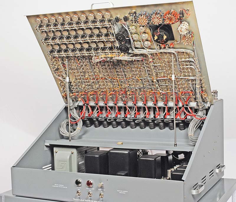
Figure 6 — Interior of the ES-400 with the front panel open, revealing the wiring harness and internal module layout. During programming, all interconnections appear on the front panel as banana-plug patch cords — the harness behind is fixed and represents the machine’s permanent internal wiring. (Reference — courtesy Nuts & Volts / David Goodsell)
5.9 Programming Tips and Common Errors
5.9.1 Checklist Before Every Run
□ All amplifiers balanced (NE-51 dark, output ≈ 0 V with shorted input)
□ IC supplies set and verified for each integrator
□ All pot settings recorded on the problem setup sheet
□ Block diagram matches physical patch — traced connection by connection
□ No NE-51 lamps lit during IC phase
□ Oscilloscope input impedance ≥ 1 MΩ
□ Power-up sequence: POWER ON → warm-up 30 min → HIGH VOLTAGE ON
□ ES-505 rate set to desired repetition frequency
5.9.2 Common Errors and Fixes
Table 19 — Common Errors and Fixes
| Symptom | Likely Cause | Fix |
|---|---|---|
| Solution grows without bound (runaway) | Sign error in feedback path | Re-check sign at every node; add or remove inverter |
| Output stuck at +100 V or −100 V | NE-51 lit — scaling error | Reduce all scale factors by factor of 2; reduce pot settings |
| Solution always zero, no response | Missing or reversed feedback patch | Trace patch cords from output back to input; check IC level |
| Oscillation at wrong frequency | Time constant mismatch | Verify Ri and Cf values; check for wrong resistor in wrong jack |
| Poor repeatability run-to-run | Amplifier not balanced, or IC supply drifting | Re-balance amps; verify IC supply output with meter |
| NE-51 flickers but does not stay lit | Transient overshoot during IC→OPERATE transition | Apply time scaling (increase β) to slow the initial transient |
| Phase-plane trace drifts slowly | Amplifier DC offset (leakage current) | Re-balance; check for leaky integration capacitor |
Note — The Operational Manual states regarding initial-condition relay bias: “In order to avoid bias, it is necessary that the relay be connected to the input of the amplifier and not to the output.” Connecting the IC supply directly to the output rather than through the relay to the input will prevent proper IC operation and produce the “always zero” symptom.
5.9.3 Sign-Check Method (Without Running the Problem)
Before committing to a run, verify the sign of the feedback loop with a static test:
- Set the OPERATE RELAY to OPERATE (not IC).
- Set all pots to minimum.
- Apply a small positive voltage (e.g., +10 V from a partial pot on the reference supply) to the input of AMP-1.
- Observe the output of the last integrator.
- Slowly connect the feedback path and observe whether the loop is negative (output moves in the direction that reduces the input — correct, stable) or positive (output moves to reinforce the input — incorrect, unstable).
A positive feedback loop produces runaway immediately; a negative feedback loop approaches a finite equilibrium.
5.9.4 Documentation Discipline
An analog computer problem cannot be “saved” in the modern software sense. The only record of a setup is the operator’s own documentation. Standard practice for each problem:
- Block diagram — labeled with amplifier numbers, signal names, and polarities.
- Component table — Ri and Cf for every amplifier.
- Patch list — every cord, from-jack to to-jack, with color.
- Pot settings table — recorded before and after each run.
- Oscilloscope photo or sketch — the result of each run.
- IC settings — voltage at each integrator IC terminal.
The Operational Manual concludes its programming section with: “Many other illustrative problems are given in the general references in the bibliography as well as in the specific references given in Appendix A.” The ES-400 Operational Manual bibliography lists Johnson (1956), Korn & Korn (1956), and several other classical analog-computer programming texts, all of which remain excellent references for extending beyond the examples provided here.
Cross-references: hardware architecture and the ES-201 amplifier circuit → Vol 2; front panel layout and jack assignments → Vol 3; restoration and alignment procedures including amplifier balancing → Vol 4; extended programming examples including oscillators, projectile motion, and nonlinear problems → Vol 6.
Comments (0)