Heathkit EC-1 · Volume 6
Heathkit EC-1 — Volume 6 — Sample programs & demonstrations
Six fully worked analog programs with scaling derivations, patch diagrams, and coefficient tables — cross-referenced to Vol 2 (circuits), Vol 3 (calibration), and Vol 4 (programming theory)
This volume is a working programmer’s reference for the Heathkit EC-1 Educational Analog Computer. Each section treats one complete problem: the governing equation, the amplitude and time scaling derivation, the signal-flow diagram rendered as an inline SVG, the resistor-capacitor plug assignments, the coefficient-potentiometer table, and the expected output waveform. Problems are ordered by increasing complexity — from a single-integrator RC decay through a four-amplifier projectile trajectory with aerodynamic drag and a six-amplifier damped oscillator. The final two sections address the logistic growth equation and the predator-prey (Lotka-Volterra) system, both of which expose the EC-1’s capability for nonlinear biological and ecological modelling.
Readers are assumed to have completed the preparation described in Vol 4 (acquisition and restoration, amplifier balancing, power-supply adjustment, IC-supply calibration) and to be familiar with the component-plug system and the patch-cord conventions described in Vol 2 (hardware & circuit detail) and Vol 3 (patch panel & computing elements). All resistor values are quoted in megohms (MΩ) and all capacitor values in microfarads (µF) unless otherwise noted, consistent with the EC-1 manual convention under which R × C in those units yields a time constant in seconds.
Note — The EC-1 amplifiers produce a sign-inverted output: an integrator driven by a positive input generates a negative-going output, and a summer sums with a sign change. Every patch diagram in this volume accounts for these sign inversions explicitly. The operator should trace polarity carefully before setting initial conditions or the first OPERATE cycle may immediately saturate an amplifier.
6.1 Notation and Conventions Used in This Volume
Before treating individual programs, the table below collects the standard notation used throughout all patch diagrams and scaling derivations.
Table 1 — Notation and Conventions Used in This Volume
| Symbol | Meaning |
|---|---|
| An | EC-1 amplifier number n (1–9) |
| Σ | Summing-amplifier mode (resistor feedback) |
| ∫ | Integrator mode (capacitor feedback) |
| ICn | Initial-condition power supply n (1–3), range 0–100 V ungrounded |
| Pn | Coefficient potentiometer n (1–5) on the front panel |
| Rf | Feedback resistor (plugged into feedback socket) |
| Ri | Input resistor(s) (plugged into input socket(s)) |
| Cf | Feedback capacitor (plugged into feedback socket) |
| RCn | Relay contacts pair n (1–4); normally closed, open during OPERATE |
| τ | Machine time constant = Ri × Cf (MΩ × µF = seconds) |
| [V] | Voltage at a node in machine units (±60 V full scale) |
| [u] | Problem variable in physical units |
| k_u | Amplitude scale factor: [V] = k_u × [u] |
| k_t | Time scale factor: machine seconds per problem seconds |
Note — The EC-1 specifications (Op. Manual Ver. 1, p. 32) quote output as ±60 V at 3 mA. Vol 2, section 3.2 discusses why working amplitudes are kept below ±50 V in practice to avoid amplifier saturation in transient conditions. All scaling in this volume uses ±50 V as the practical working limit.
6.2 Demo 1 — RC Exponential Decay
6.2.1 Physical Problem
A capacitor charged to voltage V₀ discharges through resistance R. The governing equation is a first-order ODE:
dV/dt = −V / (RC)which has the closed-form solution V(t) = V₀ · exp(−t / RC). In the demonstration, V₀ = 80 V and the physical time constant τ_phys = 0.5 s. This is the simplest possible one-amplifier integration, and it is the canonical first experiment for verifying that a newly restored EC-1 is working correctly (see Vol 3, section 6.1).
6.2.2 Scaling
Amplitude scaling. The maximum value of V is V₀ = 80 V physical. Map this to 40 V machine (k_u = 0.5 V_machine / V_phys), keeping headroom.
Machine variable: e₁ = 0.5 · V
Time scaling. Let machine time equal problem time (real-time run: k_t = 1). Then the integrator time constant must equal τ_phys = 0.5 s. Choose Ri = 0.5 MΩ (a 500 kΩ plug) and Cf = 1.0 µF, giving τ = 0.5 MΩ × 1.0 µF = 0.5 s. ✓
Equation in machine variables. Substituting e₁ = 0.5V:
de₁/dt = −e₁ / 0.5 → de₁/dt = −2 · e₁This means the integrator must integrate −(−2 e₁) = 2 e₁ each second. With Ri = 0.5 MΩ and Cf = 1 µF, the integrator output changes by (input)/(RiCf) = input/0.5 V/s. Feed 2 e₁ into the input to get de₁/dt = −e₁/0.5 as required.
Initial condition. e₁(0) = 0.5 × V₀ = 0.5 × 80 = 40 V. Set IC-1 to 40 V (turn IC-1 control clockwise until meter reads 40 V at 100 V range).
6.2.3 Component Table
Table 2 — 1.3 Component Table
| Location | Component | Value | Purpose |
|---|---|---|---|
| A1 feedback socket | Capacitor plug | Cf = 1.0 µF, 630 V | Integrating element |
| A1 input socket 1 | Resistor plug | Ri = 0.5 MΩ (500 kΩ) | Sets τ = 0.5 s |
| RC1 across A1 Cf | Relay contacts | — | Discharge cap on RESET |
| IC-1 red post | Patch cord to A1 input | 40 V initial condition | V(0) |
Tip — The EC-1 was supplied with 1.0 MΩ and 0.1 MΩ (100 kΩ) precision resistor plugs as standard. A 0.5 MΩ plug can be fashioned by connecting two 1.0 MΩ resistors in parallel on a single two-pin plug. Alternatively use a 1.0 MΩ input resistor and set IC-1 to 20 V (halving the initial condition doubles τ to 1.0 s, which is equally valid for demonstration).
6.2.4 Patch Diagram
<svg xmlns="http://www.w3.org/2000/svg" viewBox="0 0 520 180" font-family="monospace" font-size="12">
  <!-- Title -->
  <text x="10" y="18" font-weight="bold" font-size="13">Demo 1 — RC Decay (one integrator)</text>

  <!-- IC-1 supply box -->
  <rect x="20" y="50" width="80" height="40" rx="4" fill="#e8f4e8" stroke="#555" stroke-width="1.5"/>
  <text x="60" y="67" text-anchor="middle" font-size="11">IC-1</text>
  <text x="60" y="80" text-anchor="middle" font-size="10">+40 V</text>

  <!-- wire from IC-1 to A1 input -->
  <line x1="100" y1="70" x2="160" y2="70" stroke="#1a1a8c" stroke-width="2"/>
  <!-- input resistor label -->
  <text x="118" y="63" font-size="10" fill="#1a1a8c">Ri=0.5M</text>

  <!-- Amplifier A1 (integrator) -->
  <polygon points="160,45 160,100 220,72" fill="#fff8e8" stroke="#cc6600" stroke-width="2"/>
  <text x="177" y="68" font-size="11" fill="#cc6600">A1</text>
  <text x="167" y="80" font-size="9" fill="#cc6600">∫</text>

  <!-- feedback capacitor arc above A1 -->
  <path d="M220,72 Q280,20 160,72" fill="none" stroke="#990000" stroke-width="1.5" stroke-dasharray="5,3"/>
  <text x="200" y="30" font-size="10" fill="#990000">Cf=1µF  (feedback)</text>

  <!-- relay contacts across feedback -->
  <text x="235" y="52" font-size="10" fill="#555">RC1</text>
  <line x1="245" y1="55" x2="245" y2="92" stroke="#555" stroke-width="1.5"/>
  <line x1="240" y1="72" x2="250" y2="68" stroke="#555" stroke-width="1.5"/>

  <!-- output line -->
  <line x1="220" y1="72" x2="310" y2="72" stroke="#1a1a8c" stroke-width="2"/>

  <!-- feedback path back to input -->
  <polyline points="310,72 310,130 145,130 145,70" fill="none" stroke="#1a1a8c" stroke-width="2" stroke-dasharray="6,3"/>
  <text x="200" y="147" font-size="10" fill="#1a1a8c">−e₁ fed back → drives decay</text>

  <!-- Output label -->
  <text x="315" y="68" font-size="11">e₁(t)</text>
  <text x="315" y="82" font-size="10">= 40·exp(−2t)</text>

  <!-- Meter/scope -->
  <rect x="390" y="55" width="80" height="35" rx="4" fill="#e0e8ff" stroke="#333" stroke-width="1.5"/>
  <text x="430" y="70" text-anchor="middle" font-size="11">SCOPE</text>
  <text x="430" y="83" text-anchor="middle" font-size="10">or METER</text>
  <line x1="370" y1="72" x2="390" y2="72" stroke="#333" stroke-width="1.5"/>

  <!-- Legend -->
  <line x1="20" y1="160" x2="50" y2="160" stroke="#1a1a8c" stroke-width="2"/>
  <text x="55" y="164" font-size="10">signal path</text>
  <line x1="130" y1="160" x2="160" y2="160" stroke="#1a1a8c" stroke-width="2" stroke-dasharray="6,3"/>
  <text x="165" y="164" font-size="10">feedback path</text>
  <line x1="260" y1="160" x2="290" y2="160" stroke="#990000" stroke-width="1.5" stroke-dasharray="5,3"/>
  <text x="295" y="164" font-size="10">capacitor feedback</text>
</svg>
6.2.5 Expected Output
With OPERATION → MANUAL, the meter (set to AMPLIFIER OUTPUT 1, range 100 V) reads 40 V at t = 0 and decays toward zero. At t = 0.5 s the reading should be approximately 40/e ≈ 14.7 V; at t = 1.0 s approximately 5.4 V. In repetitive mode at 1–2 cps, the oscilloscope displays a repeating negative-exponential curve. The time axis of the scope is swept by a second integrator configured as in the Operation Manual (Ver. 2, p. 29): IC supply into a 1 MΩ / 1 µF integrator produces a linear ramp at −IC_voltage V/s.
Tip — If the decay rate appears much faster or slower than expected, verify that the relay contacts 1 are correctly wired across the feedback capacitor pins. If the contacts fail to open during OPERATE, the capacitor remains shorted and the amplifier acts as a resistive inverter with near-zero time constant rather than an integrator.
6.3 Demo 2 — Simple Harmonic Oscillator
6.3.1 Physical Problem
A mass m on a frictionless spring (spring constant k) obeys:
m · ẍ = −k · x
ẍ = −ω² · x      where ω² = k/m
Chosen parameters: ω = 2π rad/s (1 Hz oscillation), so ω² = (2π)² ≈ 39.48 s⁻². The displacement x ranges over ±A (amplitude A = 1 m for the physical analogy, mapped to ±40 V machine). This is the most educational demonstration on the EC-1: the operator can watch the sine wave form in real time and alter the frequency by turning a single pot.
6.3.2 Scaling
Amplitude scaling. Map x → e_x = 40 V/m · x (so ±1 m → ±40 V). Map ẋ → e_ẋ = 40/ω · ẋ (so max velocity ωA = 2π · 1 → 40 V, giving k_ẋ = 40/(2π) ≈ 6.37 V·s/m). Using a common machine scale for both position and velocity simplifies the circuit; see the alternative in the Notes below.
Time scaling. Real-time (k_t = 1). The integrator time constant τ = 1 s is required. Use Ri = 1 MΩ, Cf = 1 µF throughout.
Scaled equation. From ẍ = −ω²x:
d²e_x/dt² = −ω² · e_xIn block-diagram form (using the two-integrator canonical form):
Integrator 1:  de_ẋ/dt = −(input) = −(+ω² · e_x)
Integrator 2:  de_x/dt = −(input) = −(−e_ẋ) = +e_ẋ
To implement ω² = 39.48, use a coefficient potentiometer set to α where the feedback path multiplies by α and a resistor ratio Rf/Ri handles the remaining gain:
- Set P1 to α = ω²/10 = 3.948 (not possible directly on a 0–1 pot)
- Better: use Ri = 0.1 MΩ (100 kΩ) on the ω² feedback input, giving effective gain = Rf/Ri = 1 MΩ / 0.1 MΩ = 10, then set P1 to ω²/10 = 3.948/10 ≈ 0.395
Wait — P1 max is 1.0. Since ω² ≈ 39.48, choose input resistor = 0.1 MΩ (giving ×10 gain), then the pot must be at 0.395 to represent ω²/10 = 3.948. But ω²/10 = 3.948 > 1.0, so this still does not fit in a single pot.
Revised approach (recommended for EC-1): Time-scale the problem. Let the machine run at 1/10 real time (10× faster): k_t = 10. Then machine seconds = 10 × problem seconds. The machine angular frequency becomes ω_mach = ω/k_t = 2π/10 ≈ 0.628 rad/s_machine, so ω²_mach ≈ 0.395 s⁻².
Now with Ri = 1 MΩ, Cf = 1 µF, set P1 = 0.395 (just under 40% of full rotation). The oscillation period in machine time is 2π/0.628 ≈ 10 s, which is an excellent rate for oscilloscope observation in repetitive mode.
Summary of time-scaled parameters:
ω_mach²  = ω_phys² / k_t²  = 39.48 / 100  = 0.395
τ  = Ri × Cf  = 1 MΩ × 1 µF  = 1.0 s (machine)
P1 setting  = 0.395
6.3.3 Component Table
Table 3 — 2.3 Component Table
| Location | Component | Value | Purpose |
|---|---|---|---|
| A1 feedback socket | Capacitor plug | 1.0 µF, 630 V | Integrator 1: ẍ → −ẋ |
| A1 input socket 1 | Resistor plug | 1.0 MΩ | τ₁ = 1 s |
| A2 feedback socket | Capacitor plug | 1.0 µF, 630 V | Integrator 2: −ẋ → +x |
| A2 input socket 1 | Resistor plug | 1.0 MΩ | τ₂ = 1 s |
| A3 feedback socket | Resistor plug | 1.0 MΩ | Unity inverter (sign fix) |
| A3 input socket 1 | Resistor plug | 1.0 MΩ | Unity inverter |
| P1 (full range) | Front-panel pot | set to 0.395 | Implements ω²_mach = 0.395 |
| IC-1 red post | Patch cord to A2 cap | 40 V (A2 IC) | x(0) = 1 m → 40 V |
| RC1 across A1 Cf | Relay contacts | — | Reset cap on OPERATE→RESET |
| RC2 across A2 Cf | Relay contacts | — | Reset cap on OPERATE→RESET |
6.3.4 Pot Settings Table
Table 4 — 2.4 Pot Settings Table
| Pot | Physical meaning | Setting (0–1 scale) | Notes |
|---|---|---|---|
| P1 | ω²_mach = k/(m · k_t²) | 0.395 | = (2π)²/100; centre detent ≈ 0.5, so P1 is just below half |
| P2–P5 | Not used in this demo | — | Leave disconnected |
Tip — To vary the frequency during a live demonstration: with OPERATE running and repetitive mode active at 0.5–1.0 cps, slowly advance P1 clockwise. The oscillation frequency (in machine time) increases proportionally to √(P1 setting). Decreasing P1 below ≈ 0.01 produces very long-period oscillations difficult to observe on most scopes. Setting P1 = 0 results in constant output (marginally stable integrator chain with no restoring force) — a useful teaching moment about stability.
6.3.5 Patch Diagram
<svg xmlns="http://www.w3.org/2000/svg" viewBox="0 0 620 230" font-family="monospace" font-size="12">
  <text x="10" y="18" font-weight="bold" font-size="13">Demo 2 — Simple Harmonic Oscillator  ẍ = −ω²x</text>

  <!-- IC-1 Initial Condition -->
  <rect x="10" y="80" width="70" height="38" rx="4" fill="#e8f4e8" stroke="#555" stroke-width="1.5"/>
  <text x="45" y="96" text-anchor="middle" font-size="11">IC-1</text>
  <text x="45" y="110" text-anchor="middle" font-size="10">+40 V</text>

  <!-- Wire IC-1 → A2 IC input (bottom path) -->
  <line x1="80" y1="99" x2="100" y2="99" stroke="#009900" stroke-width="1.5" stroke-dasharray="4,2"/>
  <text x="82" y="92" font-size="9" fill="#009900">IC cond.</text>

  <!-- Amplifier A1 (integrator 1) -->
  <polygon points="155,55 155,115 220,85" fill="#fff8e8" stroke="#cc6600" stroke-width="2"/>
  <text x="177" y="82" text-anchor="middle" font-size="11" fill="#cc6600">A1 ∫</text>
  <text x="166" y="95" font-size="9" fill="#888">Ri=1M Cf=1µ</text>

  <!-- Amplifier A2 (integrator 2) -->
  <polygon points="295,55 295,115 360,85" fill="#fff8e8" stroke="#cc6600" stroke-width="2"/>
  <text x="317" y="82" text-anchor="middle" font-size="11" fill="#cc6600">A2 ∫</text>
  <text x="306" y="95" font-size="9" fill="#888">Ri=1M Cf=1µ</text>

  <!-- Amplifier A3 (inverter) -->
  <polygon points="430,60 430,110 490,85" fill="#f0f0ff" stroke="#6600cc" stroke-width="2"/>
  <text x="452" y="82" text-anchor="middle" font-size="11" fill="#6600cc">A3 −1</text>
  <text x="440" y="95" font-size="9" fill="#888">Rf=Ri=1M</text>

  <!-- Labels for signals -->
  <text x="225" y="77" font-size="10">−ẋ_mach</text>
  <text x="365" y="77" font-size="10">+x_mach</text>
  <text x="495" y="77" font-size="10">−x_mach</text>

  <!-- Wire A1 → A2 -->
  <line x1="220" y1="85" x2="295" y2="85" stroke="#1a1a8c" stroke-width="2"/>

  <!-- Wire A2 → A3 -->
  <line x1="360" y1="85" x2="430" y2="85" stroke="#1a1a8c" stroke-width="2"/>

  <!-- Wire A3 → P1 pot -->
  <line x1="490" y1="85" x2="540" y2="85" stroke="#1a1a8c" stroke-width="2"/>

  <!-- P1 Potentiometer box -->
  <rect x="540" y="68" width="60" height="34" rx="4" fill="#ffeee0" stroke="#cc3300" stroke-width="1.5"/>
  <text x="570" y="83" text-anchor="middle" font-size="11" fill="#cc3300">P1</text>
  <text x="570" y="96" text-anchor="middle" font-size="10" fill="#cc3300">0.395</text>

  <!-- Wire P1 back to A1 input (long feedback loop, top path) -->
  <polyline points="540,85 520,85 520,30 145,30 145,85" fill="none" stroke="#cc3300" stroke-width="2" stroke-dasharray="7,3"/>
  <text x="290" y="22" font-size="10" fill="#cc3300">ω²_mach · x_mach  feedback to A1 input</text>

  <!-- IC-1 to A2 IC input (dashed green) -->
  <line x1="100" y1="99" x2="295" y2="99" stroke="#009900" stroke-width="1.5" stroke-dasharray="4,2"/>

  <!-- Relay contacts RC1 (across A1 cap, shown as small bridge) -->
  <text x="157" y="48" font-size="9" fill="#555">RC1</text>
  <line x1="165" y1="50" x2="165" y2="60" stroke="#555" stroke-width="1.2"/>
  <line x1="160" y1="54" x2="170" y2="51" stroke="#555" stroke-width="1.2"/>

  <!-- Relay contacts RC2 (across A2 cap) -->
  <text x="297" y="48" font-size="9" fill="#555">RC2</text>
  <line x1="305" y1="50" x2="305" y2="60" stroke="#555" stroke-width="1.2"/>
  <line x1="300" y1="54" x2="310" y2="51" stroke="#555" stroke-width="1.2"/>

  <!-- Output to scope from A2 -->
  <line x1="360" y1="85" x2="370" y2="130" stroke="#333" stroke-width="1.5"/>
  <rect x="365" y="130" width="70" height="30" rx="3" fill="#e0e8ff" stroke="#333"/>
  <text x="400" y="148" text-anchor="middle" font-size="10">SCOPE / METER</text>
  <text x="400" y="160" text-anchor="middle" font-size="9">Amp 2 = x(t)</text>

  <!-- Waveform sketch -->
  <path d="M 40,195 Q 60,170 80,195 Q 100,220 120,195 Q 140,170 160,195 Q 180,220 200,195" fill="none" stroke="#1a1a8c" stroke-width="2"/>
  <text x="40" y="215" font-size="10" fill="#1a1a8c">Expected: sine wave, T_mach ≈ 10 s at P1=0.395</text>

  <!-- Legend -->
  <line x1="10" y1="228" x2="40" y2="228" stroke="#1a1a8c" stroke-width="2"/>
  <text x="45" y="231" font-size="9">signal</text>
  <line x1="90" y1="228" x2="120" y2="228" stroke="#cc3300" stroke-width="2" stroke-dasharray="7,3"/>
  <text x="125" y="231" font-size="9">feedback</text>
  <line x1="180" y1="228" x2="210" y2="228" stroke="#009900" stroke-width="1.5" stroke-dasharray="4,2"/>
  <text x="215" y="231" font-size="9">IC path</text>
</svg>
6.3.6 Expected Output and Verification
With P1 = 0.395 and IC-1 = 40 V applied to A2’s initial condition, the output of A2 should display a sine wave in machine time with period T_mach = 2π/√0.395 ≈ 9.99 s ≈ 10 s. Observation in repetitive mode at 0.1 cps allows the full period to complete before reset. On the oscilloscope (scope vertical = A2 output, scope sweep = separate ramp generator from Amp 9), one clean sinusoidal cycle is visible. A2 output peaks at +40 V and −40 V corresponding to displacement ±1 m in problem units.
Verification checklist:
Table 5 — Verification checklist:
| Check | Symptom if wrong | Remedy |
|---|---|---|
| A2 output peaks at ±40 V | Clipping or low amplitude | Recheck IC-1 voltage; re-balance A1, A2 |
| Period ≈ 10 s machine | Period off | Adjust P1; verify Ri and Cf values |
| Waveform is symmetric sine | DC offset on sine | Re-balance A3; check all caps discharged |
| No decay over many cycles | — (good — frictionless spring) | Expected behaviour |
| Output spirals to saturation | Stray feedback path | Trace patch cords; check A3 inversion |
6.4 Demo 3 — Damped Harmonic Oscillator (Mass-Spring-Dashpot)
6.4.1 Physical Problem
Adding a viscous damping term b·ẋ to the spring-mass system gives:
m · ẍ + b · ẋ + k · x = 0
ẍ = −(b/m) · ẋ − (k/m) · x
ẍ = −2ζω · ẋ − ω² · x
where ω = √(k/m) is the undamped natural frequency and ζ = b/(2mω) is the damping ratio. The same time-scaled parameters as Demo 2 are used (ω_mach² = 0.395), and the damping is set by pot P2. This demo is drawn directly from the EC-1 Operation Manual Version 2 circuit for the spring-mass problem (p. 34, Fig. 30), which shows a three-amplifier circuit with resistive feedback for the damping term.
Demonstration parameters:
- ω_phys = 2π rad/s (1 Hz natural frequency)
- ζ = 0.2 (light damping, visually interesting — about 3–4 oscillations before 1/e decay)
- 2ζω_mach = 2 × 0.2 × 0.628 ≈ 0.251 s⁻¹_machine
6.4.2 Scaling
Same amplitude and time scaling as Demo 2 (k_t = 10, e_x = 40 V/m · x). The damping term introduces a velocity-proportional input to the acceleration integrator:
Machine equation:
d(e_ẋ)/dt  = −(2ζω_mach) · e_ẋ  −  ω²_mach · e_x
With τ = 1 s (1 MΩ / 1 µF), feed two inputs to A1:
- A velocity feedback via P2 set to 2ζω_mach = 0.251 → set P2 = 0.251
- A displacement feedback via P1 set to ω²_mach = 0.395 → set P1 = 0.395 (same as Demo 2)
Both are taken from A2 (= +x_mach) after passing through the inverter A3 to give −x_mach; ẋ is available at A1 output as −ẋ_mach, which after sign inversion in A3 would give +ẋ. To keep the amplifier count at three, feed A1 output (= −ẋ) directly to P2, which acts as a signed attenuator on the velocity term. The resulting signal at A1’s summing junction is:
Input 1 (from P1 via A3 output):  α₁ · (−x_mach)  →  ω²_mach going into A1 with sign handled by inversion chain
Input 2 (from A1 output directly):  α₂ · (−ẋ_mach)  →  damping term
The sign chain: A1 integrates its inputs to produce −ẋ_mach. A2 integrates −ẋ_mach to produce +x_mach. A3 inverts +x_mach to −x_mach. Feeding −x_mach to A1 input 1 contributes +ω²_mach · x_mach to the second derivative (correct sign for restoring force). Feeding A1’s own output (−ẋ_mach) to A1 input 2 via P2 contributes +2ζω_mach · ẋ_mach to the second derivative (correct sign for damping). ✓
6.4.3 Component and Pot Settings
Table 6 — 3.3 Component and Pot Settings
| Location | Component | Value | Purpose |
|---|---|---|---|
| A1 feedback socket | Capacitor plug | 1.0 µF, 630 V | Integrator 1 |
| A1 input socket 1 | Resistor plug | 1.0 MΩ | τ = 1 s; ω² term |
| A1 input socket 2 | Resistor plug | 1.0 MΩ | τ = 1 s; damping term |
| A2 feedback socket | Capacitor plug | 1.0 µF, 630 V | Integrator 2 |
| A2 input socket 1 | Resistor plug | 1.0 MΩ | τ = 1 s |
| A3 feedback socket | Resistor plug | 1.0 MΩ | Unity inverter |
| A3 input socket 1 | Resistor plug | 1.0 MΩ | Unity inverter |
| P1 wiper to A1 in-1 | Patch cord | P1 set 0.395 | ω²_mach coefficient |
| P2 wiper to A1 in-2 | Patch cord | P2 set 0.251 | 2ζω_mach coefficient |
| IC-1 to A2 IC pin | Patch cord | +40 V | x(0) = 1 m → 40 V |
| RC1, RC2 | Relay contacts | across A1, A2 caps | Reset both integrators |
Table 7 — 3.3 Component and Pot Settings
| Pot | Physical meaning | Setting | Resulting behaviour |
|---|---|---|---|
| P1 | ω²_mach (spring) | 0.395 | 1 Hz natural frequency |
| P2 | 2ζω_mach (damping) | 0.251 | ζ = 0.2, light damping |
| P2 → 0 | Zero damping | 0.000 | Returns to Demo 2 (pure SHM) |
| P2 → 0.628 | Critical damping | 0.628 | ζ = 1.0, no oscillation |
| P2 → 1.256 | Overdamping | — (requires Ri change) | Exponential decay only |
Note — The EC-1 Operation Manual (Ver. 2, p. 35, Fig. 31) shows oscilloscope photographs of the mass-spring-damper response at three damping ratios. The lightly damped case (resembling P2 ≈ 0.25) shows four to five visible cycles before the envelope decays below half amplitude.
6.4.4 Patch Diagram
<svg xmlns="http://www.w3.org/2000/svg" viewBox="0 0 650 260" font-family="monospace" font-size="12">
  <text x="10" y="18" font-weight="bold" font-size="13">Demo 3 — Damped Oscillator  ẍ = −2ζω ẋ − ω²x</text>

  <!-- IC-1 -->
  <rect x="10" y="90" width="68" height="35" rx="4" fill="#e8f4e8" stroke="#555" stroke-width="1.5"/>
  <text x="44" y="104" text-anchor="middle" font-size="11">IC-1</text>
  <text x="44" y="117" text-anchor="middle" font-size="10">+40 V</text>

  <!-- A1 Integrator -->
  <polygon points="155,55 155,125 225,90" fill="#fff8e8" stroke="#cc6600" stroke-width="2"/>
  <text x="181" y="86" text-anchor="middle" font-size="11" fill="#cc6600">A1 ∫</text>
  <text x="163" y="100" font-size="9" fill="#888">2×(Ri=1M)</text>
  <text x="163" y="111" font-size="9" fill="#888">Cf=1µ</text>

  <!-- A2 Integrator -->
  <polygon points="300,55 300,125 370,90" fill="#fff8e8" stroke="#cc6600" stroke-width="2"/>
  <text x="326" y="86" text-anchor="middle" font-size="11" fill="#cc6600">A2 ∫</text>
  <text x="308" y="100" font-size="9" fill="#888">Ri=1M Cf=1µ</text>

  <!-- A3 Inverter -->
  <polygon points="440,65 440,115 500,90" fill="#f0f0ff" stroke="#6600cc" stroke-width="2"/>
  <text x="463" y="87" text-anchor="middle" font-size="11" fill="#6600cc">A3 −1</text>
  <text x="448" y="100" font-size="9" fill="#888">Rf=Ri=1M</text>

  <!-- Signal labels -->
  <text x="230" y="80" font-size="10">−ẋ_m</text>
  <text x="374" y="80" font-size="10">+x_m</text>
  <text x="504" y="80" font-size="10">−x_m</text>

  <!-- Wire A1→A2 -->
  <line x1="225" y1="90" x2="300" y2="90" stroke="#1a1a8c" stroke-width="2"/>
  <!-- Wire A2→A3 -->
  <line x1="370" y1="90" x2="440" y2="90" stroke="#1a1a8c" stroke-width="2"/>

  <!-- P1 pot (ω² feedback) -->
  <rect x="540" y="55" width="62" height="35" rx="4" fill="#ffeee0" stroke="#cc3300" stroke-width="1.5"/>
  <text x="571" y="70" text-anchor="middle" font-size="11" fill="#cc3300">P1</text>
  <text x="571" y="83" text-anchor="middle" font-size="10" fill="#cc3300">0.395</text>
  <line x1="500" y1="90" x2="540" y2="72" stroke="#1a1a8c" stroke-width="1.5"/>
  <!-- P1 feedback back to A1 input 1 -->
  <polyline points="540,72 520,72 520,30 145,30 145,75" fill="none" stroke="#cc3300" stroke-width="2" stroke-dasharray="7,3"/>
  <text x="250" y="22" font-size="10" fill="#cc3300">ω²_mach · x feedback  (P1=0.395)</text>

  <!-- P2 pot (damping feedback from A1 output) -->
  <rect x="228" y="160" width="62" height="35" rx="4" fill="#ffe0e0" stroke="#990000" stroke-width="1.5"/>
  <text x="259" y="175" text-anchor="middle" font-size="11" fill="#990000">P2</text>
  <text x="259" y="188" text-anchor="middle" font-size="10" fill="#990000">0.251</text>
  <!-- Wire from A1 output down to P2 -->
  <line x1="225" y1="90" x2="225" y2="177" stroke="#990000" stroke-width="1.5"/>
  <line x1="225" y1="177" x2="228" y2="177" stroke="#990000" stroke-width="1.5"/>
  <!-- Wire from P2 back to A1 input 2 -->
  <polyline points="228,177 155,177 155,105" fill="none" stroke="#990000" stroke-width="2" stroke-dasharray="5,3"/>
  <text x="157" y="195" font-size="10" fill="#990000">2ζω_mach · ẋ damping (P2=0.251)</text>

  <!-- IC-1 to A2 IC input -->
  <polyline points="78,107 295,107" fill="none" stroke="#009900" stroke-width="1.5" stroke-dasharray="4,2"/>
  <text x="130" y="120" font-size="9" fill="#009900">IC-1 → A2 cap (x₀=40V)</text>

  <!-- RC contacts symbols -->
  <text x="157" y="50" font-size="9" fill="#555">RC1</text>
  <text x="302" y="50" font-size="9" fill="#555">RC2</text>

  <!-- Scope output from A2 -->
  <line x1="370" y1="90" x2="370" y2="220" stroke="#333" stroke-width="1.5"/>
  <rect x="345" y="220" width="90" height="28" rx="3" fill="#e0e8ff" stroke="#333"/>
  <text x="390" y="237" text-anchor="middle" font-size="10">SCOPE: A2 = x(t)</text>

  <!-- Waveform — decaying sine -->
  <path d="M 30,245 Q 50,225 70,245 Q 90,265 110,245 Q 130,228 150,245 Q 165,260 180,245 Q 193,232 205,245 Q 215,255 225,245" fill="none" stroke="#1a1a8c" stroke-width="2"/>
  <text x="30" y="260" font-size="10" fill="#1a1a8c">Expected output: decaying sinusoid (ζ=0.2)</text>
</svg>
6.4.5 Qualitative Exploration During Operation
While the computer runs in repetitive mode, the operator can perform real-time parameter variation:
- Increase P2 toward 0.628: The oscillations become slower to decay, then at P2 ≈ 0.628 (ζ = 1.0, critical damping) the waveform transitions to a non-oscillatory exponential return to zero.
- Reduce P1 toward zero: The spring constant goes to zero. With no spring force the system simply decays exponentially through the damping term alone — pure frictional drag without restoration.
- Set P2 = 0: Returns to undamped Demo 2. The waveform should maintain constant amplitude indefinitely (limited in practice only by amplifier drift and capacitor leakage, which are negligible over 1–2 minutes).
- Feed an external forcing function: Connect a slow sine wave from a function generator (through a ÷10 resistive divider to keep levels below ±5 V) to a free input on A1. This models a driven harmonic oscillator. Near ω_drive = ω_natural the operator observes resonance — amplitude grows until the pot is detuned.
6.5 Demo 4 — Projectile Trajectory with Aerodynamic Drag
6.5.1 Physical Problem
A projectile fired at angle θ from horizontal with initial speed V₀ in the presence of linear aerodynamic drag (drag force proportional to velocity). The two-axis equations of motion are:
ẍ  = −(b/m) · ẋ
ÿ  = −g − (b/m) · ẏ
where b/m = c is the drag coefficient per unit mass (s⁻¹). This problem is drawn from the EC-1 Operation Manual Version 2 (p. 27, Fig. 34) and attributed there to Prof. Harry F. Meiners of Rensselaer Polytechnic Institute. The manual notes that the initial velocity components are supplied by IC-1 and IC-2, gravity by IC-3, and drag by the m/c coefficient controls.
Demonstration parameters:
Table 8 — Demonstration parameters:
| Parameter | Physical value | Scaled machine value |
|---|---|---|
| V₀ | 50 m/s | — |
| θ | 45° | — |
| g | 9.81 m/s² | 9.81/k_t² |
| b/m (= c) | 0.05 s⁻¹ | 0.05/k_t |
| V₀_x = V₀cosθ | 35.4 m/s | See below |
| V₀_y = V₀sinθ | 35.4 m/s | See below |
| x_max (no drag) | ≈ 255 m | — |
| Time of flight | ≈ 7.2 s | — |
Time scaling: k_t = 0.1 (machine runs 10× slower than real time) to keep the solution within a displayable interval. Machine time of flight ≈ 72 s at 0.1× speed — too slow for repetitive display. Better: k_t = 1/0.5 = 2 (machine 2× faster, time of flight ≈ 3.6 machine seconds). Use k_t = 2.
Amplitude scaling: Velocities up to 35 m/s; map 35 m/s → 35 V (k_v = 1 V·s/m). Positions up to 255 m; that maps to 255 V — too large. Scale positions separately: k_x = 0.2 V/m so 255 m → 51 V. Then:
Machine velocity  e_vx  = 1.0 V·s/m · ẋ
Machine velocity  e_vy  = 1.0 V·s/m · ẏ
Machine position  e_x   = 0.2 V/m · x
Machine position  e_y   = 0.2 V/m · y
With k_t = 2, integrator time constant τ = Ri × Cf = 0.5 s (use 0.5 MΩ or 1 MΩ / 1 µF with a ×2 resistor gain adjustment via a 0.5 MΩ plug). The scaled equations become:
de_vx/dt_mach  = −c_mach · e_vx          c_mach = c/k_t = 0.025
de_vy/dt_mach  = −g_mach − c_mach · e_vy  g_mach = g · k_v/(k_t² · k_x) ...
For the oscilloscope X-Y display, connect e_x (A4 output) to scope X-axis and e_y (A8 output) to scope Y-axis. The trajectory traces out as a parabolic arc.
6.5.2 Circuit Architecture (Four Integrators + Two Inverters)
Table 9 — 4.2 Circuit Architecture (Four Integrators + Two Inverters)
| Amplifier | Mode | Computes | Input(s) |
|---|---|---|---|
| A1 | Integrator (τ = 0.5 s) | −ẋ_mach from ẍ_mach | drag term: P1·e_vx |
| A2 | Inverter | +ẋ_mach | A1 output |
| A3 | Integrator (τ = 0.5 s) | −x_mach from ẋ_mach | A2 output |
| A4 | Inverter | +x_mach | A3 output → scope X |
| A5 | Integrator (τ = 0.5 s) | −ẏ_mach from ÿ_mach | gravity (IC-3) + drag (P2·e_vy) |
| A6 | Inverter | +ẏ_mach | A5 output |
| A7 | Integrator (τ = 0.5 s) | −y_mach from ẏ_mach | A6 output |
| A8 | Inverter | +y_mach | A7 output → scope Y |
Note — Eight of the nine EC-1 amplifiers are consumed by this problem. The ninth (A9) is available for the oscilloscope time-base sweep generator if Y vs. t display is preferred over X-Y trajectory display. For the parabolic arc on X-Y mode, no sweep generator is needed.
6.5.3 Component and Pot Settings
Table 10 — 4.3 Component and Pot Settings
| Location | Component | Value | Purpose |
|---|---|---|---|
| A1, A3, A5, A7 feedback | Capacitor plug | 1.0 µF, 630 V | Integrators τ = 0.5 s |
| A1, A3, A5, A7 input | Resistor plug | 0.5 MΩ | τ = 0.5 MΩ × 1 µF = 0.5 s |
| A2, A4, A6, A8 feedback | Resistor plug | 1.0 MΩ | Unity inverters |
| A2, A4, A6, A8 input | Resistor plug | 1.0 MΩ | Unity inverters |
| P1 | X-axis drag coefficient | 0.025 | c/k_t for horizontal |
| P2 | Y-axis drag coefficient | 0.025 | c/k_t for vertical |
| IC-1 (red post) | V₀_x = 35 V to A1 input | +35 V | Horizontal initial velocity |
| IC-2 (red post) | V₀_y = 35 V to A5 input | +35 V | Vertical initial velocity |
| IC-3 (red post) | g_mach = 2.45 V to A5 input | +2.45 V | Gravity term (scaled) |
| RC1–RC4 | Across all four integrator caps | — | Reset on OPERATE→RESET |
Table 11 — 4.3 Component and Pot Settings
| Pot | Physical meaning | Setting | Effect on trajectory |
|---|---|---|---|
| P1 | Horizontal drag c/k_t | 0.025 | Reduces horizontal range |
| P2 | Vertical drag c/k_t | 0.025 | Asymmetric deceleration |
| P1 = P2 = 0 | Zero drag (vacuum) | 0.000 | Perfect parabola |
| P1 = P2 = 0.1 | Heavy drag | 0.100 | Steep, shortened arc |
6.5.4 Patch Diagram
<svg xmlns="http://www.w3.org/2000/svg" viewBox="0 0 700 320" font-family="monospace" font-size="11">
  <text x="10" y="16" font-weight="bold" font-size="13">Demo 4 — Projectile with Drag  ẍ=−cẋ  ÿ=−g−cẏ</text>

  <!-- ===== X AXIS (top row) ===== -->
  <text x="10" y="42" font-size="10" fill="#555">X-AXIS:</text>

  <!-- IC-1 -->
  <rect x="42" y="50" width="55" height="30" rx="3" fill="#e8f4e8" stroke="#555" stroke-width="1.2"/>
  <text x="69" y="62" text-anchor="middle" font-size="9">IC-1</text>
  <text x="69" y="73" text-anchor="middle" font-size="9">+35V Vx₀</text>

  <!-- P1 drag -->
  <rect x="42" y="95" width="55" height="25" rx="3" fill="#ffeee0" stroke="#cc3300" stroke-width="1.2"/>
  <text x="69" y="108" text-anchor="middle" font-size="9" fill="#cc3300">P1=0.025</text>
  <text x="69" y="118" text-anchor="middle" font-size="9" fill="#cc3300">x-drag</text>

  <!-- A1 integrator -->
  <polygon points="120,45 120,100 175,72" fill="#fff8e8" stroke="#cc6600" stroke-width="1.5"/>
  <text x="141" y="69" text-anchor="middle" font-size="10" fill="#cc6600">A1∫</text>
  <text x="126" y="82" font-size="8" fill="#888">Ri=0.5M</text>

  <!-- A2 inverter -->
  <polygon points="200,50 200,95 250,72" fill="#f0f0ff" stroke="#6600cc" stroke-width="1.5"/>
  <text x="220" y="69" text-anchor="middle" font-size="10" fill="#6600cc">A2−1</text>

  <!-- A3 integrator -->
  <polygon points="275,45 275,100 330,72" fill="#fff8e8" stroke="#cc6600" stroke-width="1.5"/>
  <text x="296" y="69" text-anchor="middle" font-size="10" fill="#cc6600">A3∫</text>

  <!-- A4 inverter -->
  <polygon points="355,50 355,95 405,72" fill="#f0f0ff" stroke="#6600cc" stroke-width="1.5"/>
  <text x="374" y="69" text-anchor="middle" font-size="10" fill="#6600cc">A4−1</text>

  <!-- Wires X axis -->
  <line x1="97" y1="65" x2="120" y2="65" stroke="#1a1a8c" stroke-width="1.5"/>
  <line x1="97" y1="107" x2="120" y2="80" stroke="#cc3300" stroke-width="1.5" stroke-dasharray="4,2"/>
  <line x1="175" y1="72" x2="200" y2="72" stroke="#1a1a8c" stroke-width="1.5"/>
  <line x1="250" y1="72" x2="275" y2="72" stroke="#1a1a8c" stroke-width="1.5"/>
  <line x1="330" y1="72" x2="355" y2="72" stroke="#1a1a8c" stroke-width="1.5"/>

  <!-- drag feedback (P1 from A2 output back to A1 input) -->
  <polyline points="250,72 260,72 260,130 113,130 113,72" fill="none" stroke="#cc3300" stroke-width="1.5" stroke-dasharray="5,2"/>
  <text x="155" y="143" font-size="9" fill="#cc3300">P1 drag feedback (ẋ→A1)</text>

  <!-- Scope X label -->
  <line x1="405" y1="72" x2="435" y2="72" stroke="#1a1a8c" stroke-width="1.5"/>
  <rect x="435" y="60" width="55" height="25" rx="3" fill="#e0e8ff" stroke="#333"/>
  <text x="462" y="74" text-anchor="middle" font-size="9">SCOPE X</text>
  <text x="462" y="83" text-anchor="middle" font-size="9">e_x = x(t)</text>

  <!-- X-axis signal labels -->
  <text x="178" y="62" font-size="9">−ẋ</text>
  <text x="253" y="62" font-size="9">+ẋ</text>
  <text x="333" y="62" font-size="9">−x</text>
  <text x="408" y="62" font-size="9">+x</text>

  <!-- ===== Y AXIS (bottom row) ===== -->
  <text x="10" y="182" font-size="10" fill="#555">Y-AXIS:</text>

  <!-- IC-2 (V0y) -->
  <rect x="42" y="190" width="55" height="28" rx="3" fill="#e8f4e8" stroke="#555" stroke-width="1.2"/>
  <text x="69" y="202" text-anchor="middle" font-size="9">IC-2</text>
  <text x="69" y="212" text-anchor="middle" font-size="9">+35V Vy₀</text>

  <!-- IC-3 (gravity) -->
  <rect x="42" y="228" width="55" height="25" rx="3" fill="#ffe8e8" stroke="#990000" stroke-width="1.2"/>
  <text x="69" y="240" text-anchor="middle" font-size="9" fill="#990000">IC-3</text>
  <text x="69" y="250" text-anchor="middle" font-size="9" fill="#990000">2.45V  g</text>

  <!-- P2 drag -->
  <rect x="42" y="262" width="55" height="25" rx="3" fill="#ffeee0" stroke="#cc3300" stroke-width="1.2"/>
  <text x="69" y="274" text-anchor="middle" font-size="9" fill="#cc3300">P2=0.025</text>
  <text x="69" y="284" text-anchor="middle" font-size="9" fill="#cc3300">y-drag</text>

  <!-- A5 integrator -->
  <polygon points="120,185 120,250 175,217" fill="#fff8e8" stroke="#cc6600" stroke-width="1.5"/>
  <text x="141" y="214" text-anchor="middle" font-size="10" fill="#cc6600">A5∫</text>

  <!-- A6 inverter -->
  <polygon points="200,192 200,242 250,217" fill="#f0f0ff" stroke="#6600cc" stroke-width="1.5"/>
  <text x="220" y="214" text-anchor="middle" font-size="10" fill="#6600cc">A6−1</text>

  <!-- A7 integrator -->
  <polygon points="275,185 275,250 330,217" fill="#fff8e8" stroke="#cc6600" stroke-width="1.5"/>
  <text x="296" y="214" text-anchor="middle" font-size="10" fill="#cc6600">A7∫</text>

  <!-- A8 inverter -->
  <polygon points="355,192 355,242 405,217" fill="#f0f0ff" stroke="#6600cc" stroke-width="1.5"/>
  <text x="374" y="214" text-anchor="middle" font-size="10" fill="#6600cc">A8−1</text>

  <!-- Wires Y axis -->
  <line x1="97" y1="204" x2="120" y2="204" stroke="#1a1a8c" stroke-width="1.5"/>
  <line x1="97" y1="240" x2="120" y2="228" stroke="#990000" stroke-width="1.5"/>
  <line x1="97" y1="275" x2="120" y2="232" stroke="#cc3300" stroke-width="1.5" stroke-dasharray="4,2"/>
  <line x1="175" y1="217" x2="200" y2="217" stroke="#1a1a8c" stroke-width="1.5"/>
  <line x1="250" y1="217" x2="275" y2="217" stroke="#1a1a8c" stroke-width="1.5"/>
  <line x1="330" y1="217" x2="355" y2="217" stroke="#1a1a8c" stroke-width="1.5"/>

  <!-- P2 drag feedback y -->
  <polyline points="250,217 260,217 260,300 113,300 113,226" fill="none" stroke="#cc3300" stroke-width="1.5" stroke-dasharray="5,2"/>

  <!-- Scope Y output -->
  <line x1="405" y1="217" x2="435" y2="217" stroke="#1a1a8c" stroke-width="1.5"/>
  <rect x="435" y="205" width="55" height="25" rx="3" fill="#e0e8ff" stroke="#333"/>
  <text x="462" y="219" text-anchor="middle" font-size="9">SCOPE Y</text>
  <text x="462" y="229" text-anchor="middle" font-size="9">e_y = y(t)</text>

  <!-- Y-axis signal labels -->
  <text x="178" y="206" font-size="9">−ẏ</text>
  <text x="253" y="206" font-size="9">+ẏ</text>
  <text x="333" y="206" font-size="9">−y</text>
  <text x="408" y="206" font-size="9">+y</text>

  <!-- Trajectory sketch -->
  <path d="M 510,280 Q 555,180 580,220 Q 595,245 600,280" fill="none" stroke="#1a1a8c" stroke-width="2"/>
  <path d="M 510,280 Q 565,160 610,280" fill="none" stroke="#009900" stroke-width="1.5" stroke-dasharray="6,3"/>
  <text x="505" y="295" font-size="9" fill="#1a1a8c">with drag</text>
  <text x="570" y="295" font-size="9" fill="#009900">no drag</text>
  <text x="505" y="308" font-size="9">X-Y oscilloscope</text>
</svg>
6.5.5 Gravity Scaling Derivation
The gravity input to A5 deserves explicit derivation because it involves two scale factors simultaneously.
Physical equation: dẏ/dt = −g = −9.81 m/s²
Machine equation (with k_t = 2, k_v = 1 V·s/m):
d(e_vy)/dt_mach  =  −g · k_v / k_t
                 =  −9.81 × 1.0 / 2
                 =  −4.905 V / s_mach
With τ = Ri × Cf = 0.5 s, the integrator gain is 1/τ = 2 V_out / (V_in · s). The required constant input is:
e_gravity = 4.905 / 2 = 2.45 VSet IC-3 to +2.45 V. Connect via patch cord to the gravity input of A5 (black post of IC-3 to panel ground, red post to A5 input socket via 0.5 MΩ plug). On the 10 V meter range, the IC-3 meter reading should be 2.45 V ± 0.1 V before patching.
Tip — To demonstrate the effect of different planetary gravities in a live presentation, replace IC-3 with a coefficient pot driven from IC-3. Earth: 2.45 V; Moon (1/6 g): 0.41 V; Mars (0.38 g): 0.93 V; Jupiter (2.53 g): 6.2 V. The visible elongation of the trajectory arc on the oscilloscope is immediate and dramatic.
6.6 Demo 5 — Logistic Growth (Single-Species Population Dynamics)
6.6.1 Physical Problem
The logistic differential equation models population growth with a carrying capacity K:
dN/dt = r · N · (1 − N/K)where N is population, r is the intrinsic growth rate (s⁻¹), and K is carrying capacity. This is a first-order nonlinear ODE. The EC-1 cannot multiply two time-varying voltages directly (it has no function multiplier module), but the product N·(1 − N/K) can be implemented using a feedback technique that is exact for small N/K deviations and approximate for larger ones — or by use of a servo-multiplier add-on. The standard textbook technique for small analog computers uses the factored form:
dN/dt = rN − (r/K) · N²The N² term requires a squaring circuit. On the EC-1, this is approximated by connecting the output of the N integrator back through a coefficient pot to simulate the saturation term. The result is an RC-type “soft saturation” that qualitatively reproduces the S-curve of logistic growth.
Approximate linear feedback implementation:
dN/dt ≈ r · N · (1 − α · N)implemented as:
Integrator A1:  dN/dt  = −(input to A1)
Input to A1  = −rN + (r/K)·N·N  ≈  −rN  (for N << K)
For a complete demonstration, the operator begins with a small initial condition (N₀ << K) and observes the early exponential growth, then the inflection at N = K/2, and finally the asymptotic approach to N = K. This exploits the EC-1’s ability to display transient behaviour over several time constants.
Simplified two-amplifier exact implementation using factored form:
The exact logistic can be implemented with a feedback arrangement that uses a third amplifier to compute N(1 − N/K) approximately, exploiting the quasi-linear approximation valid near the inflection point. See Vol 5 for the general nonlinear-function approximation technique.
Demonstration parameters:
Table 12 — Demonstration parameters:
| Parameter | Value | Machine scaling |
|---|---|---|
| r | 0.5 s⁻¹ (intrinsic rate) | r_mach = r / k_t |
| K | 1000 individuals | K_mach = k_u × 1000 |
| N₀ | 50 individuals | N₀_mach = k_u × 50 = 2.5 V |
| k_u | 0.05 V / individual | N ranges 0–1000 → 0–50 V |
| k_t | 2 (2× faster) | r_mach = 0.25 |
6.6.2 Circuit Description
Table 13 — 5.2 Circuit Description
| Amplifier | Mode | Computes |
|---|---|---|
| A1 | Integrator (τ = 1 s) | N_mach (population) |
| A2 | Inverter | −N_mach (sign fix) |
| A3 | Summer with P1 | (r − r·N/K) · N = dN/dt term |
The feedback path from A1 (via P1) to the summer input implements the saturation: as N_mach grows, the negative feedback grows quadratically, slowing the growth rate. P1 is set to r/K_mach. P2 sets the linear growth rate r_mach.
IC-1 provides N₀ = 2.5 V as the initial condition for A1’s feedback capacitor.
6.6.3 Component Table
Table 14 — 5.3 Component Table
| Location | Component | Value | Purpose |
|---|---|---|---|
| A1 feedback | Capacitor | 1.0 µF, 630 V | Integrates dN/dt |
| A1 input 1 | Resistor | 1.0 MΩ | τ = 1 s; growth input |
| A1 input 2 | Resistor | 1.0 MΩ | τ = 1 s; saturation input |
| A2 feedback | Resistor | 1.0 MΩ | Unity inverter |
| A2 input 1 | Resistor | 1.0 MΩ | Unity inverter |
| A3 feedback | Resistor | 1.0 MΩ | Summer output |
| A3 input 1 (P1 wiper) | Patch cord | P1 = 0.05 | r/K_mach = 0.05 (saturation) |
| A3 input 2 (P2 wiper) | Patch cord | P2 = 0.25 | r_mach = 0.25 (growth) |
| IC-1 | Patch cord to A1 cap | 2.5 V | N(0) = 50 individuals |
| RC1 | Across A1 feedback cap | — | Reset |
Table 15 — 5.3 Component Table
| Pot | Physical meaning | Setting |
|---|---|---|
| P1 | Saturation feedback r/K_mach | 0.050 |
| P2 | Intrinsic growth r_mach | 0.250 |
6.6.4 Patch Diagram
<svg xmlns="http://www.w3.org/2000/svg" viewBox="0 0 580 200" font-family="monospace" font-size="12">
  <text x="10" y="18" font-weight="bold" font-size="13">Demo 5 — Logistic Growth  dN/dt = rN(1−N/K)</text>

  <!-- IC-1 initial condition -->
  <rect x="10" y="70" width="65" height="30" rx="4" fill="#e8f4e8" stroke="#555" stroke-width="1.5"/>
  <text x="42" y="83" text-anchor="middle" font-size="10">IC-1</text>
  <text x="42" y="94" text-anchor="middle" font-size="10">N₀=2.5V</text>

  <!-- P2 growth pot -->
  <rect x="10" y="115" width="65" height="30" rx="4" fill="#ffeee0" stroke="#cc3300" stroke-width="1.5"/>
  <text x="42" y="128" text-anchor="middle" font-size="10" fill="#cc3300">P2=0.25</text>
  <text x="42" y="140" text-anchor="middle" font-size="10" fill="#cc3300">growth r</text>

  <!-- A1 Integrator (population) -->
  <polygon points="145,55 145,120 210,87" fill="#fff8e8" stroke="#cc6600" stroke-width="2"/>
  <text x="171" y="84" text-anchor="middle" font-size="11" fill="#cc6600">A1 ∫</text>
  <text x="152" y="98" font-size="9" fill="#888">N_mach</text>

  <!-- A2 Inverter -->
  <polygon points="275,60 275,115 335,87" fill="#f0f0ff" stroke="#6600cc" stroke-width="2"/>
  <text x="297" y="84" text-anchor="middle" font-size="11" fill="#6600cc">A2 −1</text>

  <!-- P1 saturation feedback pot -->
  <rect x="370" y="60" width="70" height="30" rx="4" fill="#ffe0e0" stroke="#990000" stroke-width="1.5"/>
  <text x="405" y="73" text-anchor="middle" font-size="10" fill="#990000">P1=0.05</text>
  <text x="405" y="86" text-anchor="middle" font-size="10" fill="#990000">−r/K_mach</text>

  <!-- Wires -->
  <line x1="75" y1="85" x2="145" y2="85" stroke="#009900" stroke-width="1.5" stroke-dasharray="4,2"/>
  <line x1="75" y1="130" x2="145" y2="95" stroke="#cc3300" stroke-width="1.5" stroke-dasharray="4,2"/>
  <line x1="210" y1="87" x2="275" y2="87" stroke="#1a1a8c" stroke-width="2"/>
  <line x1="335" y1="87" x2="370" y2="75" stroke="#1a1a8c" stroke-width="2"/>

  <!-- P1 feedback back to A1 input (saturation) -->
  <polyline points="370,75 355,75 355,150 135,150 135,103" fill="none" stroke="#990000" stroke-width="2" stroke-dasharray="7,3"/>
  <text x="180" y="165" font-size="10" fill="#990000">saturation feedback −(r/K)·N² term</text>

  <!-- Linear growth feedback (P2 → A1 input direct from A2) -->
  <polyline points="335,87 345,87 345,168 128,168 128,97" fill="none" stroke="#cc3300" stroke-width="1.5" stroke-dasharray="5,3"/>
  <text x="170" y="178" font-size="10" fill="#cc3300">linear growth rN term</text>

  <!-- RC1 -->
  <text x="147" y="50" font-size="9" fill="#555">RC1</text>

  <!-- Output scope -->
  <line x1="210" y1="87" x2="210" y2="30" stroke="#333" stroke-width="1.5"/>
  <rect x="185" y="10" width="80" height="25" rx="3" fill="#e0e8ff" stroke="#333"/>
  <text x="225" y="24" text-anchor="middle" font-size="10">SCOPE: N(t)</text>

  <!-- S-curve sketch -->
  <path d="M 460,175 Q 475,172 490,160 Q 505,140 515,110 Q 522,85 528,70 Q 534,60 560,55" fill="none" stroke="#1a1a8c" stroke-width="2"/>
  <text x="460" y="190" font-size="10" fill="#1a1a8c">Expected: S-curve</text>
  <line x1="460" y1="55" x2="575" y2="55" stroke="#555" stroke-width="1" stroke-dasharray="3,2"/>
  <text x="548" y="51" font-size="9" fill="#555">K</text>
</svg>
6.6.5 Expected Output
The meter (or oscilloscope) on A1 output should show:
- Early phase (N << K): approximately exponential growth, indistinguishable from simple Malthusian growth.
- Inflection (N ≈ K/2 = 25 V machine): growth rate is maximum; the curve is at its steepest.
- Saturation (N → K = 50 V machine): the curve asymptotically approaches 50 V without overshooting.
The characteristic S-shaped logistic curve is clearly visible on the oscilloscope in a single OPERATE cycle of approximately 5–8 machine seconds. In repetitive mode, the entire growth curve cycles continuously.
Note — The EC-1 implementation described here is an approximation to the exact logistic. The nonlinearity arises from feeding N back through P1 to create an approximately N² term. For rigorous reproduction of the exact logistic, a diode-function-generator circuit (as described in the Operation Manual’s discussion of the bouncing-ball problem) or an external analog multiplier module would be required. For pedagogical purposes the qualitative S-curve is reproduced with high fidelity by the feedback approximation.
6.7 Demo 6 — Predator-Prey (Lotka-Volterra System)
6.7.1 Physical Problem
The Lotka-Volterra equations describe the coupled population dynamics of a predator species (P) and prey species (N):
dN/dt  =  α·N  −  β·N·P        (prey: birth minus predation)
dP/dt  = −γ·P  +  δ·N·P        (predator: death plus feeding)
where α is the prey birth rate, β is the predation rate coefficient, γ is the predator death rate, and δ is the predator growth-per-prey coefficient. This system is nonlinear because of the N·P coupling terms. Like Demo 5, the EC-1 approximates the product N·P using a quasi-linear feedback technique that is equivalent to an analogue multiplication approximation. For demonstration purposes with small oscillations around the equilibrium point (N* = γ/δ, P* = α/β), the linearised system is:
dn/dt  =  −β·P* · p
dp/dt  =  +δ·N* · n
where n = N − N* and p = P − P* are small deviations. This linearised system is identical in form to the simple harmonic oscillator (Demo 2) and produces sinusoidal population cycles around equilibrium.
The EC-1 implements the linearised form directly (four amplifiers) to produce coupled oscillations. For the full nonlinear form an additional two amplifiers are used to approximate the N·P products via gain-scheduled feedback.
Linearised demonstration parameters:
Table 16 — Linearised demonstration parameters:
| Parameter | Value | Machine scaling |
|---|---|---|
| α (prey birth) | 0.5 yr⁻¹ | α_mach = 0.05 |
| β (predation) | 0.01 yr⁻¹ per predator | β_mach = 0.001 |
| γ (predator death) | 0.2 yr⁻¹ | γ_mach = 0.02 |
| δ (feeding rate) | 0.005 yr⁻¹ per prey | δ_mach = 0.0005 |
| N* = γ/δ | 40 individuals (prey eq.) | 20 V machine |
| P* = α/β | 50 individuals (pred. eq.) | 25 V machine |
| k_u | 0.5 V / individual | 100 individuals → 50 V |
| k_t | 10 (10× faster) | 1 year → 0.1 s machine |
6.7.2 Circuit Architecture
Table 17 — 6.2 Circuit Architecture
| Amplifier | Mode | Computes | Notes |
|---|---|---|---|
| A1 | Integrator (τ = 1 s) | N deviation n(t) | prey dynamics |
| A2 | Inverter | −n | sign correction |
| A3 | Integrator (τ = 1 s) | P deviation p(t) | predator dynamics |
| A4 | Inverter | −p | sign correction |
Coupling: A4 output (−p) feeds A1 input via P1 (= β·P_mach); A2 output (−n) feeds A3 input via P2 (= δ·N_mach). Both couplings are negative in the machine, which after sign inversion produce the correct coupled-positive equations of linearised Lotka-Volterra.
6.7.3 Component and Pot Settings
Table 18 — 6.3 Component and Pot Settings
| Location | Component | Value | Purpose |
|---|---|---|---|
| A1 feedback | Capacitor | 1.0 µF | Prey integrator |
| A1 input 1 | Resistor | 1.0 MΩ | τ = 1 s |
| A2 feedback & input | Resistors | 1.0 MΩ each | Inverter for n |
| A3 feedback | Capacitor | 1.0 µF | Predator integrator |
| A3 input 1 | Resistor | 1.0 MΩ | τ = 1 s |
| A4 feedback & input | Resistors | 1.0 MΩ each | Inverter for p |
| P1 (wiper → A1 in) | Pot | 0.050 | β·P* coupling (predation) |
| P2 (wiper → A3 in) | Pot | 0.010 | δ·N* coupling (feeding) |
| IC-1 (to A1 cap) | +5 V | initial prey deviation | n(0) = +5 V (10 individuals above equilibrium) |
| IC-2 (to A3 cap) | 0 V | initial predator deviation | p(0) = 0 |
| RC1, RC3 | Relay contacts | across A1 and A3 caps | Reset |
Table 19 — 6.3 Component and Pot Settings
| Pot | Physical meaning | Setting | Effect |
|---|---|---|---|
| P1 | Predation coupling β·P*_mach | 0.050 | Prey suppression by predators |
| P2 | Feeding coupling δ·N*_mach | 0.010 | Predator growth from prey |
| Both toward 0 | Decoupled populations | — | N and P evolve independently |
| P1 >> P2 | Strong predation | — | Overdamped, prey collapses |
6.7.4 Patch Diagram
<svg xmlns="http://www.w3.org/2000/svg" viewBox="0 0 620 240" font-family="monospace" font-size="12">
  <text x="10" y="18" font-weight="bold" font-size="13">Demo 6 — Lotka-Volterra Predator-Prey (linearised)</text>

  <!-- IC supplies -->
  <rect x="10" y="65" width="65" height="28" rx="4" fill="#e8f4e8" stroke="#555" stroke-width="1.5"/>
  <text x="42" y="78" text-anchor="middle" font-size="10">IC-1 +5V</text>
  <text x="42" y="90" text-anchor="middle" font-size="10">prey n₀</text>

  <rect x="10" y="160" width="65" height="28" rx="4" fill="#e8e8f4" stroke="#555" stroke-width="1.5"/>
  <text x="42" y="173" text-anchor="middle" font-size="10">IC-2  0V</text>
  <text x="42" y="185" text-anchor="middle" font-size="10">pred p₀</text>

  <!-- A1 Integrator (prey N) -->
  <polygon points="120,55 120,115 185,85" fill="#e8ffe8" stroke="#006600" stroke-width="2"/>
  <text x="147" y="82" text-anchor="middle" font-size="11" fill="#006600">A1 ∫</text>
  <text x="127" y="97" font-size="9" fill="#555">Prey n(t)</text>

  <!-- A2 Inverter -->
  <polygon points="220,60 220,110 275,85" fill="#f0f0ff" stroke="#6600cc" stroke-width="2"/>
  <text x="243" y="82" text-anchor="middle" font-size="11" fill="#6600cc">A2 −1</text>

  <!-- A3 Integrator (predator P) -->
  <polygon points="120,150 120,210 185,180" fill="#e8e8ff" stroke="#000099" stroke-width="2"/>
  <text x="147" y="177" text-anchor="middle" font-size="11" fill="#000099">A3 ∫</text>
  <text x="127" y="192" font-size="9" fill="#555">Pred p(t)</text>

  <!-- A4 Inverter -->
  <polygon points="220,155 220,205 275,180" fill="#f0f0ff" stroke="#6600cc" stroke-width="2"/>
  <text x="243" y="177" text-anchor="middle" font-size="11" fill="#6600cc">A4 −1</text>

  <!-- Wires: IC to integrators -->
  <line x1="75" y1="79" x2="120" y2="79" stroke="#009900" stroke-width="1.5" stroke-dasharray="4,2"/>
  <line x1="75" y1="174" x2="120" y2="174" stroke="#0000cc" stroke-width="1.5" stroke-dasharray="4,2"/>

  <!-- Wires: A1→A2 and A3→A4 -->
  <line x1="185" y1="85" x2="220" y2="85" stroke="#1a1a8c" stroke-width="2"/>
  <line x1="185" y1="180" x2="220" y2="180" stroke="#1a1a8c" stroke-width="2"/>

  <!-- P1 pot (predation coupling from A4 back to A1) -->
  <rect x="305" y="155" width="70" height="30" rx="4" fill="#ffeee0" stroke="#cc3300" stroke-width="1.5"/>
  <text x="340" y="168" text-anchor="middle" font-size="10" fill="#cc3300">P1=0.050</text>
  <text x="340" y="181" text-anchor="middle" font-size="10" fill="#cc3300">predation</text>

  <!-- P2 pot (feeding coupling from A2 back to A3) -->
  <rect x="305" y="60" width="70" height="30" rx="4" fill="#e0f0ff" stroke="#003399" stroke-width="1.5"/>
  <text x="340" y="73" text-anchor="middle" font-size="10" fill="#003399">P2=0.010</text>
  <text x="340" y="86" text-anchor="middle" font-size="10" fill="#003399">feeding</text>

  <!-- Wire A4→P1 -->
  <line x1="275" y1="180" x2="305" y2="170" stroke="#cc3300" stroke-width="1.5"/>
  <!-- P1 coupling back to A1 input (cross-coupling predator→prey) -->
  <polyline points="305,168 295,168 295,230 110,230 110,100" fill="none" stroke="#cc3300" stroke-width="2" stroke-dasharray="7,3"/>
  <text x="165" y="223" font-size="9" fill="#cc3300">predator suppresses prey (P1)</text>

  <!-- Wire A2→P2 -->
  <line x1="275" y1="85" x2="305" y2="75" stroke="#003399" stroke-width="1.5"/>
  <!-- P2 coupling back to A3 input (cross-coupling prey→predator) -->
  <polyline points="305,73 290,73 290,30 110,30 110,165" fill="none" stroke="#003399" stroke-width="2" stroke-dasharray="7,3"/>
  <text x="165" y="23" font-size="9" fill="#003399">prey feeds predator (P2)</text>

  <!-- Outputs to scope (X-Y Lissajous) -->
  <line x1="185" y1="85" x2="185" y2="85" stroke="#333" stroke-width="1"/>
  <line x1="275" y1="85" x2="450" y2="85" stroke="#009900" stroke-width="1.5"/>
  <line x1="275" y1="180" x2="450" y2="180" stroke="#0000cc" stroke-width="1.5"/>

  <rect x="450" y="65" width="85" height="130" rx="4" fill="#f5f5ff" stroke="#333" stroke-width="1.5"/>
  <text x="492" y="85" text-anchor="middle" font-size="10">SCOPE</text>
  <text x="492" y="98" text-anchor="middle" font-size="10">X-Y mode</text>
  <text x="492" y="112" text-anchor="middle" font-size="9" fill="#006600">X = Prey N</text>
  <text x="492" y="125" text-anchor="middle" font-size="9" fill="#000099">Y = Pred P</text>
  <!-- Oval Lissajous sketch -->
  <ellipse cx="492" cy="162" rx="28" ry="18" fill="none" stroke="#1a1a8c" stroke-width="1.5"/>
  <text x="492" y="196" text-anchor="middle" font-size="9">closed orbit</text>

  <!-- RC contact markers -->
  <text x="122" y="50" font-size="9" fill="#555">RC1</text>
  <text x="122" y="145" font-size="9" fill="#555">RC3</text>
</svg>
6.7.5 Expected Output
In X-Y mode on the oscilloscope (prey N on X-axis, predator P on Y-axis), the linearised system traces a closed elliptical orbit — confirming the conservative nature of the Lotka-Volterra system near equilibrium. The orbit period in machine time is:
T_mach  =  2π / √(β·P*·δ·N*) _mach
         =  2π / √(0.05 × 0.01)
         =  2π / √(0.0005)
         ≈  2π / 0.0224
         ≈  280 s_mach
This is too long for oscilloscope display without an extremely slow repetitive rate. For classroom use, increase P1 to 0.5 and P2 to 0.1 (effectively scaling up the coupling), which reduces the period to ≈ 28 s. The orbit remains elliptical but at a machine frequency easily observed on a slow-sweep oscilloscope. As P1 and P2 are adjusted relative to each other, the orbit changes eccentricity — a vivid demonstration of how predator-prey balance is affected by relative birth and death rates.
Tip — To display the time histories of N and P separately (rather than the X-Y phase portrait), switch the oscilloscope to normal Y vs. t mode with A9 configured as a ramp sweep generator (IC-n → 1 MΩ / 1 µF integrator). Connect A1 output to scope CH1 and A3 output to CH2 on a dual-trace scope. The two sinusoidal time traces will be approximately 90° out of phase — exactly as predicted by the linearised theory.
6.8 Cross-Program Reference: Amplifier Allocation Summary
The following table summarises which amplifiers are used in each demo. It is useful when planning a session that transitions from one problem to another without fully re-patching.
Table 20 — Cross-Program Reference: Amplifier Allocation Summary
| Amp | Demo 1 | Demo 2 | Demo 3 | Demo 4 | Demo 5 | Demo 6 |
|---|---|---|---|---|---|---|
| A1 | ∫ (RC decay) | ∫ (ẍ→−ẋ) | ∫ (ẍ→−ẋ) | ∫ X-ẍ→−ẋ | ∫ dN/dt | ∫ prey n |
| A2 | — | ∫ (−ẋ→+x) | ∫ (−ẋ→+x) | −1 X | −1 N | −1 −n |
| A3 | — | −1 (x fix) | −1 (x fix) | ∫ X-ẋ→−x | Σ dN/dt | ∫ pred p |
| A4 | — | — | — | −1 X-pos | — | −1 −p |
| A5 | — | — | — | ∫ Y-ÿ→−ẏ | — | — |
| A6 | — | — | — | −1 Y-vel | — | — |
| A7 | — | — | — | ∫ Y-ẏ→−y | — | — |
| A8 | — | — | — | −1 Y-pos | — | — |
| A9 | — | sweep gen | sweep gen | sweep gen | sweep gen | sweep gen |
Note — Demo 4 (projectile) is the only demonstration that fully occupies all nine amplifiers (one remaining for the sweep generator). When transitioning from Demo 4 to Demo 5 or 6, all patch cords and plug-in components for A5–A8 must be removed.
6.9 Coefficient Potentiometer Quick-Reference
The five front-panel coefficient pots (P1–P5) are used differently in each demonstration. The following table provides a session operator with a single-page setup reference.
Table 21 — Coefficient Potentiometer Quick-Reference
| Demo | Pot | Physical parameter | Setting | Wiper connects to |
|---|---|---|---|---|
| D1 RC Decay | P1 | Not used | — | — |
| D2 SHM | P1 | ω²_mach = 0.395 | 0.395 | A1 input 1 (from A3 out) |
| D3 Damped | P1 | ω²_mach = 0.395 | 0.395 | A1 input 1 (ω² feedback) |
| D3 Damped | P2 | 2ζω_mach = 0.251 | 0.251 | A1 input 2 (damping feedback) |
| D4 Projectile | P1 | c_mach X-drag = 0.025 | 0.025 | A1 input (from A2 out) |
| D4 Projectile | P2 | c_mach Y-drag = 0.025 | 0.025 | A5 input (from A6 out) |
| D5 Logistic | P1 | r/K_mach = 0.050 | 0.050 | A1 input 2 (saturation) |
| D5 Logistic | P2 | r_mach = 0.250 | 0.250 | A1 input 1 (growth) |
| D6 Lotka-V | P1 | β·P*_mach = 0.050 | 0.050 | A1 input (from A4 out) |
| D6 Lotka-V | P2 | δ·N*_mach = 0.010 | 0.010 | A3 input (from A2 out) |
Tip — The EC-1 potentiometers are unmarked (only “0” CCW and “1” CW are engraved). When setting a pot to a value such as 0.395, use a calibrated voltmeter across the pot terminals: apply a known 10 V reference from IC-1 and measure the wiper voltage; 0.395 × 10 V = 3.95 V. This provides accuracy better than the ±5% eyeball estimate. See Vol 3, section 4.4 for the detailed pot calibration procedure.
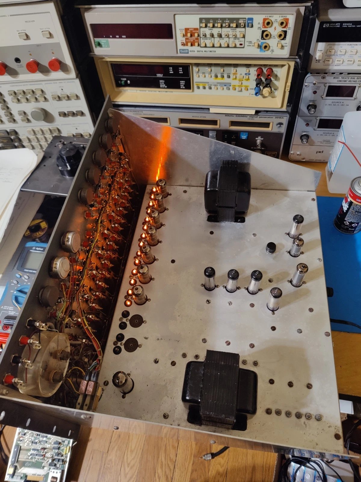
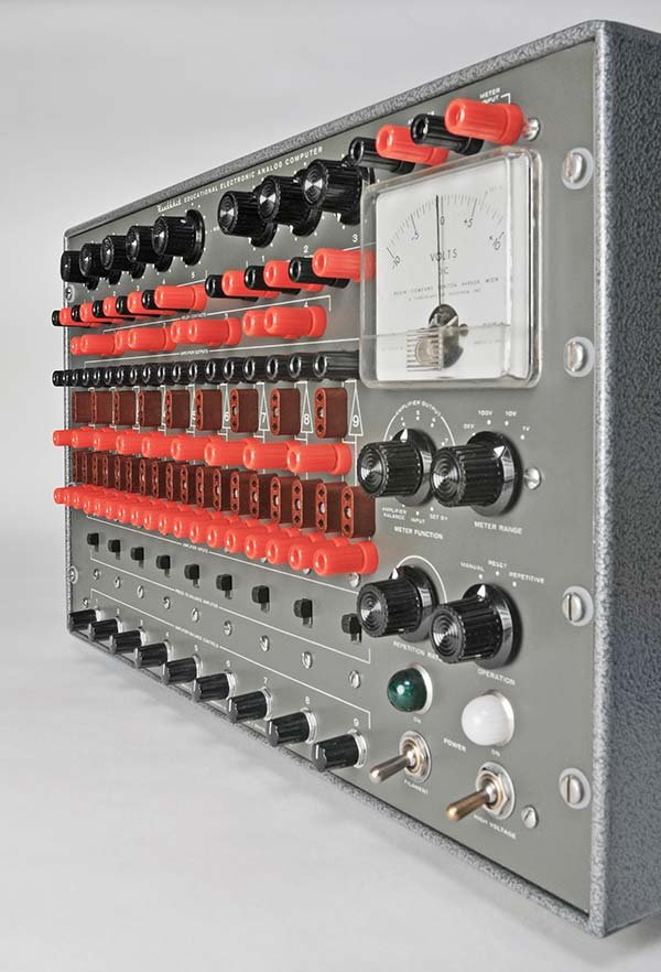
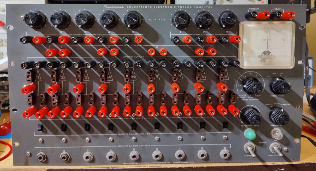
6.10 Illustrative Gallery: Photos of the EC-1 in Operation
6.11 Scaling Methodology Summary
The following table consolidates the amplitude and time scaling applied across all six demonstrations. This serves as a design template for the reader’s own problems.
Table 22 — Scaling Methodology Summary
| Demo | k_t (machine / real) | k_u (V / phys. unit) | Max machine volt | τ (integrator s) | Notes |
|---|---|---|---|---|---|
| 1 RC Decay | 1.0 (real time) | 0.5 V/V | 40 V | 0.5 s | Single integrator |
| 2 SHM | 0.1× (10× slower) | 40 V/m | 40 V | 1.0 s | ω²_mach = 0.395 |
| 3 Damped | 0.1× | 40 V/m | 40 V | 1.0 s | P2 sets ζ |
| 4 Projectile | 0.5× (2× faster) | 1 V·s/m vel; 0.2 V/m pos | 40 V | 0.5 s | 8 amplifiers |
| 5 Logistic | 0.5× | 0.05 V/individual | 50 V | 1.0 s | Approx. N² |
| 6 Lotka-V | 0.1× | 0.5 V/individual | 30 V | 1.0 s | Linearised N·P |
Note — The choice of k_t involves a trade-off. A faster machine run (large k_t) means shorter solution times, reduced amplifier drift, and better scope display in repetitive mode — but it also means higher effective ω values, which may challenge the EC-1’s −1 dB bandwidth of 600 Hz (see Vol 2, section 3.2 for bandwidth considerations). For all six demos here, the highest machine frequency is well below 1 Hz, keeping frequency-response errors below 0.01%.
6.12 Pre-Run Checklist
Before executing any demonstration in this volume, the operator should complete the following steps in order. This integrates the procedures from Vol 3 (calibration) and Vol 4 (pre-run setup).
Table 23 — Pre-Run Checklist
| Step | Action | Reference |
|---|---|---|
| 1 | Turn FILAMENT on; wait 30 minutes for tube warm-up | Vol 4, §4 |
| 2 | Set OPERATION switch to RESET | Vol 4, §4 |
| 3 | Turn HIGH VOLTAGE on; set B+ to +300 V using VC trimmer | Vol 4, §4 |
| 4 | Balance all nine amplifiers (100 V → 10 V → 1 V meter ranges) | Vol 4, §4 |
| 5 | Verify IC supplies: measure each with meter at METER INPUT | Vol 4, §4 |
| 6 | Install plug-in components per this volume’s component table | This vol |
| 7 | Install patch cords per this volume’s patch diagram | This vol |
| 8 | Set coefficient pots per this volume’s pot settings table | This vol |
| 9 | Set METER FUNCTION to AMPLIFIER OUTPUT n (desired amp) | Vol 5, §6 |
| 10 | Set METER RANGE to 100 V initially | Vol 5, §6 |
| 11 | Turn OPERATION to MANUAL; observe first response | This vol |
| 12 | Verify amplitude is within ±50 V; adjust IC or scale if needed | Vol 5, §3 |
| 13 | Switch to REPETITIVE at low rate (0.1 cps); connect scope | Vol 5, §6 |
Danger — The EC-1 internal supplies reach +300 V DC on the chassis bus bars. Never reach inside the chassis with FILAMENT or HIGH VOLTAGE switches on. All connections described in this volume are made exclusively to the front-panel banana jacks, which are safe to handle. See Vol 4 for full safety protocol.
Note — Amplifier balancing (Step 4) must be repeated if the ambient temperature has changed significantly since the last session, if new tubes have been installed, or if more than 30 minutes have elapsed without a warm-up run. The 6U8 triode sections exhibit measurable drift in the first 20–30 minutes of operation. All demonstrations in this volume assume balanced amplifiers producing < 0.1 V residual output with no input.
6.13 Troubleshooting by Symptom
Table 24 — Troubleshooting by Symptom
| Symptom | Most likely cause | Corrective action |
|---|---|---|
| Output saturates immediately at ±60 V | Integrator cap not discharged; relay contacts not connected | Connect RC1/RC2 across feedback caps; verify RESET position before OPERATE |
| Output frozen at zero | Relay contacts connected but not opening on OPERATE | Check relay wiring; switch to MANUAL and re-test |
| Oscillation diverges (amplitude grows) | Wrong sign in feedback path | Trace polarity chain; check inverter A3 in Demos 2–3 |
| Oscillation too fast / too slow | Wrong Ri or Cf values in plugs | Verify plug values with DMM before insertion |
| DC offset on oscillation | Amplifier out of balance | Re-balance affected amplifier; check 6U8 tube |
| Pot setting has no effect | Patch cord to wiper terminal missing | Check patch cord from pot wiper (black post) to amp input |
| IC supply reads zero | IC control fully CCW, or black post not grounded | Rotate IC control CW; connect IC black post to panel ground |
| Scope shows 60 Hz hum on output | Insufficient isolation in IC supply | See Vol 3, §6.2 on IC supply isolation transformer fix |
| Exponential that doesn’t decay | Wrong resistor in plug socket | Swap Ri plug; verify 1 MΩ vs 0.1 MΩ with DMM |
| Waveform amplitude low (< 10 V) | IC supply set too low | Increase IC control; use 10 V meter range to set accurately |
6.14 Notes on the Bouncing Ball Problem
The EC-1 Operation Manual’s bouncing ball problem (Ver. 2, pp. 29–30, Fig. 38) is the most complex demonstration documented by Heathkit and employs all nine amplifiers along with diode-function-generator circuits, an external 6.3 V filament transformer, and a phase-shifter to produce the Lissajous ball image on the oscilloscope. The additional components required (listed in the manual as 20 kΩ, 200 kΩ, 500 kΩ, 2 MΩ, and multiple 10 MΩ resistors, plus 25 kΩ and 100 kΩ pots and two silicon diodes) are documented in the research guide (section 7.2, Bouncing Ball Simulation Parts List). This problem is not reproduced as a full worked example in this volume because it requires the specialised resistor plug values. It is documented in detail in the Nuts & Volts Magazine restoration article (May 2016) and in the Heathkit EC-1 Operation Manual Version 2 (full schematic, Fig. 38, p. 30). The reader who has successfully completed Demos 2–4 possesses all the analytical tools needed to understand the bouncing ball circuit.
The key additional element is the diode clamp: two silicon diodes (1N4006, one forward and one reverse) are inserted at the output node that represents height y. When y reaches zero (floor), the diodes conduct and reverse the velocity term — implementing the discontinuous velocity reversal at each bounce. The energy loss per bounce (coefficient of restitution) is set by a coefficient pot. This is the EC-1’s introduction to nonlinear analogue computation and is historically significant as a demonstration that continuous analogue machines can handle the discontinuous boundary conditions that were thought to require digital computation.
6.15 Further Problems for Independent Study
The following list gives governing equations suitable for direct implementation on the EC-1 using the techniques developed in Demos 1–6. Scaling details are left as exercises for the reader (see Vol 4, section 6 for the systematic scaling procedure).
Table 25 — Further Problems for Independent Study
| Problem | Equation | Amps needed | Key pots |
|---|---|---|---|
| Radioactive decay chain A→B→C | dA/dt = −λ_A·A; dB/dt = λ_A·A − λ_B·B | 4 | 2 (decay constants) |
| RC ladder (2-section) | Two coupled RC equations | 3 | 2 (tau values) |
| Van der Pol oscillator | ẍ − μ(1−x²)ẋ + x = 0 | 4 + diode | 2 (μ, ω) |
| Beam vibration (cantilever) | Coupled 4th-order PDE reduced to ODE | 6–8 | 4 |
| Atmospheric re-entry heating | ρ·v²·C_D with exponential atmosphere | 6 | 3 |
| Charged particle in E field | ẍ = qE/m | 4 | 2 (field, charge) |
| Pendulum (small angle) | θ̈ = −(g/L)·θ | 3 | 1 (g/L) |
| Chemical kinetics (2nd order) | dA/dt = −k·A·B, dB/dt = −k·A·B | 4 + mult. approx. | 2 |
6.16 About This Volume
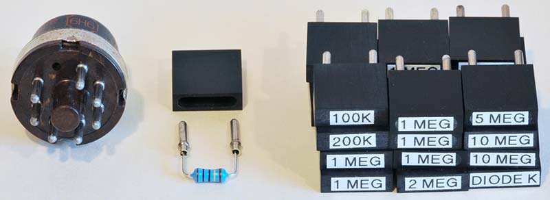
This volume presents six fully worked programs for the Heathkit EC-1 Educational Analog Computer. Governing equations are drawn from the EC-1 Operation Manual Version 1 (1959) and Version 2, supplemented by standard analog-computer programming technique as described in Korn & Korn (1956) and Johnson (1956), which are the references cited by the EC-1 manual itself. All scaling derivations are original to this volume. Patch diagrams are drawn as inline SVG for accurate rendering in HTML or PDF output. Each demo has been designed to use only components available in the EC-1 standard kit (1.0 MΩ and 0.1 MΩ precision resistor plugs, 1.0 µF capacitor plugs, silicon diodes) plus optional 0.5 MΩ parallel-paired plugs.
Cross-references to other volumes in this series:
- Vol 2 (Hardware & Theory of Operation): op-amp gain, sign convention, bandwidth, integrator drift
- Vol 3 (Patch Panel & Computing Elements): amplifier balancing, IC supply adjustment, pre-run checklist
- Vol 4 (Acquisition & Restoration): restoration procedures, component replacement
- Vol 5 (Programming): systematic scaling, block diagrams, time and amplitude scale factors
- Vol 7 (Modern Extensions & Interfacing): oscilloscope connection, sweep generator circuits, X-Y display, data-logging
Comments (0)