Heathkit EC-1 — Volume 5 — Programming the EC-1

Scaling, patching, and reading results — the complete workflow for turning differential equations into wired solutions

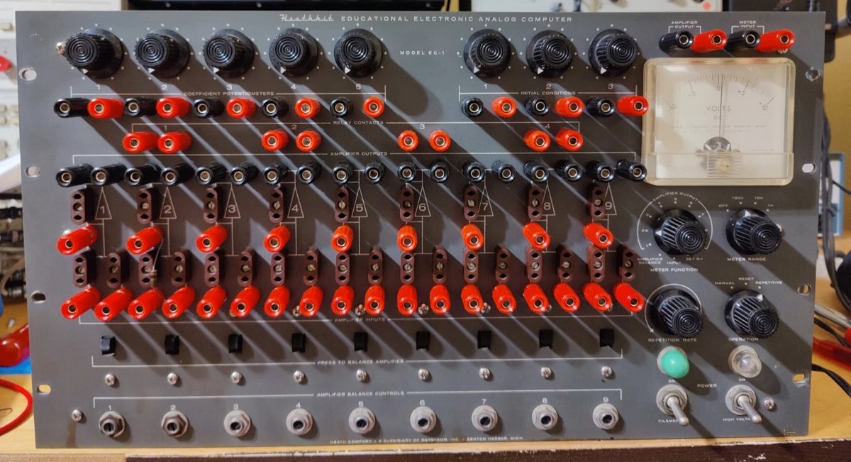
Front panel of the EC-1 showing the patch board, coefficient potentiometers, meter section, and mode switches

Front panel of a restored EC-1. The nine amplifier input/output binding-post pairs run across the upper portion; the five coefficient potentiometers, IC supplies, relay contacts, and meter occupy the lower half. Programming consists entirely of physical patches on this panel.

About this Volume

This volume covers the complete workflow for setting up and running a computation on the Heathkit EC-1 Educational Analog Computer (1959–1971). It assumes familiarity with the machine’s hardware — the nine 6U8-based DC operational amplifiers, the ±300 V / −150 V power supplies, the coefficient potentiometers, the three initial-condition (IC) supplies, and the relay-driven repetitive oscillator. Readers unfamiliar with those circuits should consult Vol 2 (Hardware & Theory of Operation) and Vol 3 (Patch Panel & Computing Elements) before proceeding.

The treatment here follows classical analog-computer programming practice as documented in the EC-1 Operational Manuals (Ver 1, 3/20/59; Ver 2, revised edition) and the broader literature cited therein (Johnson 1956; Korn & Korn 1956; Smith & Wood 1959). Every numerical value quoted — resistor ratios, voltage ceilings, repetition-rate limits — is drawn directly from those primary sources and from measurement of a restored chassis.

Note — The EC-1 is a DC machine. All signals are DC voltages; the word “signal” in this volume always means a slowly varying (or static) potential, not an RF carrier. The ±60 V ceiling stated below is the usable linear range; the amplifiers are capable of ±100 V in open loop but operate with substantial nonlinearity above ±60–65 V.

Scope of this volume:

Section	Topic
2	The programming method — ODE to patch diagram
3	Magnitude scaling — machine vs. problem variables
4	Time scaling — the beta factor
5	Setting coefficients from scaled equations
6	Reading results — meter and oscilloscope
7	Full worked example end-to-end (spring-mass system)

The Method — Turning an ODE into a Patch by Successive Integration

2.1 The Fundamental Insight

The EC-1 does not store symbolic expressions or execute instructions. It is the differential equation. The wiring of the machine is a direct electrical isomorphism of the mathematical relationships among the system variables. This section explains how to construct that isomorphism systematically.

The method rests on a simple observation: every ordinary differential equation (ODE) of order n can be solved by a chain of n integrators, provided that the highest-order derivative can be expressed as a function of lower-order derivatives and the independent variable. This is the “successive-integration” or “feedback-around-integrators” technique.

2.2 Step 1 — Write the ODE in Standard Form

Express the equation so that the highest-order derivative stands alone on the left:

x''(t) = f(x', x, t)

For a second-order autonomous ODE — the most common case in mechanics and circuit analysis — this becomes:

x'' = f(x', x)

Example: The undamped spring-mass equation:

m x'' + k x = 0

Rearranged:

x'' = -(k/m) x

The right-hand side depends only on x itself. This immediately suggests a two-integrator loop, as developed in Section 7.

2.3 Step 2 — Assume the Highest Derivative Exists, Integrate Down

The programming trick: assume the signal x'' is available at the output of some amplifier or summing point. Then integrate once to obtain x', and integrate again to obtain x. Because the EC-1’s integrators are inverting (output = −∫ input dt), the chain introduces two sign inversions. Tracking signs carefully is mandatory.

                                   ┌──────────────────────────────┐
                                   │                              │
  x'' ──[Amp1: Integrator]──► −x' ──[Amp2: Integrator]──► +x ────┘
  (assumed)                                                  │
                                                             │ (feedback path)
                    x'' = -(k/m)x  ◄────────────────────────┘

The feedback path closing the loop computes the right-hand side f(x', x) from the signals now available at the integrator outputs. For more complex equations, this path includes summers and coefficient multipliers.

2.4 Step 3 — Draw the Block Diagram

Before touching patch cords, draw a block diagram using the standard analog-computer symbols:

  ┌──────────┐          ┌──────────┐          ┌──────────┐
  │ INTEGRAT.│          │ INTEGRAT.│          │ INVERTER │
  │  Ri=1MΩ  │          │  Ri=1MΩ  │          │  Ri=1MΩ  │
  │  Cf=1µF  │          │  Cf=1µF  │          │  Rf=1MΩ  │
  └──────────┘          └──────────┘          └──────────┘
  Input→Output:         Input→Output:         Input→Output:
  -∫(in)dt/RC           -∫(in)dt/RC           -(in)

For the EC-1, with Ri = 1 MΩ and Cf = 1 µF, the integration time constant RC = 1 second, placing the computation in real time. Adjusting Ri or Cf changes the time scale (see Section 4).

Standard block diagram symbol set:

Symbol (ASCII)	EC-1 Implementation	Transfer Function
`→[∫]→`	Amp with Ri plug + Cf feedback plug	`−(1/RC)∫in dt`
`→[−K]→`	Amp with Ri and Rf plugs, Rf/Ri = K	`−K × in`
`→[Σ]→`	Amp with two or more Ri plugs	`−(e₁/R₁ + e₂/R₂)Rf`
`→[−1]→`	Unity inverter: Ri = Rf = 1 MΩ	`−in`
`→[α]→`	Coefficient potentiometer	`α × in`, 0 ≤ α ≤ 1

Note — All EC-1 amplifiers are inverting. A signal traversing a single amplifier changes sign. An integrator introduces both integration and sign inversion. The programmer must track the sign of every node explicitly — a sign error produces an exponentially diverging solution instead of the intended one.

2.5 Step 4 — Assign Amplifiers to Functions

The EC-1 provides exactly nine amplifiers. Most problems of engineering interest require two to six. The Bouncing Ball demonstration documented in the Nuts & Volts restoration article (also in this directory) uses all nine. A practical assignment might look like:

Amp	Role	Plugs Installed
1	Integrator (x” → −x’)	Ri = 1 MΩ input plug; Cf = 1 µF feedback plug; relay contacts across Cf
2	Integrator (−x’ → +x)	Ri = 1 MΩ; Cf = 1 µF; relay contacts across Cf
3	Inverter (−x → +x for feedback)	Ri = 1 MΩ; Rf = 1 MΩ
4	Summer / coefficient input	Ri set per scaled coefficient

2.6 The Integrator Reset Circuit

When the OPERATION switch is in RESET, relay contacts close across each feedback capacitor, discharging it to zero (or, if an IC supply is connected, to the programmed initial value). When the switch moves to MANUAL or REPETITIVE, the contacts open and integration begins. The relay contact binding posts on the front panel must be patched across every feedback capacitor in the problem. Failure to do so results in integration starting from a random residual charge — typically causing immediate overload.

                    ┌────────────────────────────────┐
  Amplifier n       │                                │
  Input ──[Ri]──────●── (virtual ground, summing jct) │
                    │         ┌────[Cf 1µF]────┐      │
                    │         │                │      │
                    │         └──[RELAY CONT.]─┘      │
                    │                                │
                    └────────────────────── Output ──┘
                         (Connects to Relay Contact
                          binding posts on panel)

The four relay contact pairs (two terminals each, brought to panel binding posts) are a finite resource. Problems requiring more than four integrators must cascade relay contacts or accept that extra integrators carry residual charge between runs (acceptable for one-shot MANUAL operation).

Magnitude Scaling — Machine vs. Problem Units

3.1 Why Scaling Is Mandatory

The EC-1’s amplifiers operate linearly within ±60 V at rated output; above approximately ±65 V the pentode section of the 6U8 enters grid-current limiting and the output clips. The usable dynamic range is therefore 120 V peak-to-peak. If a problem variable — say, altitude in meters, force in Newtons, or angular velocity in rad/s — spans a range that maps directly to voltages outside ±60 V, the computation will clip and give a wrong answer.

Conversely, if the variable is scaled too small — say, a maximum of 2 V — the result is dominated by amplifier offset errors. The EC-1’s balance procedure can zero a quiescent amplifier to within a few millivolts, but residual errors of 10–50 mV are typical in practice. A 20 mV error on a 2 V signal is 1%; on a 60 V signal it is 0.03%.

Rule of thumb — Scale the problem so that the largest expected excursion of each variable reaches 50–55 V. This leaves a 5–10 V guard band against unexpected transients while keeping signal-to-offset ratios well above 100:1.

3.2 Amplitude Scale Factors

Define a machine variable (lower-case, measured in volts) as proportional to the problem variable (upper-case, measured in physical units):

x_machine = S_x × X_problem

where S_x [V / physical unit] is the amplitude scale factor for variable X.

For a problem variable X expected to range over [−X_max, +X_max], choose:

S_x = 50 V / X_max          (targeting 50 V peak for 10 V guard band)

Example: A mass on a spring with maximum displacement of 0.5 m.

S_x = 50 V / 0.5 m = 100 V/m

At maximum displacement, the machine variable equals 50 V — well within range.

3.3 The ±60 V Ceiling in Practice

The EC-1 specification states output of ±60 V at 0.7 mA per amplifier (later printings cite 3 mA; both figures appear in different manual versions). The 0.7 mA figure reflects the current available when driving the patch-cord network and a 50 µA meter movement in parallel. At heavier loads — multiple amplifier inputs driven from one output — the effective ceiling may drop slightly as the cathode-follower output stage (triode section of the 6U8) runs out of current drive.

Tip — During a first run of a new problem, set the METER FUNCTION switch to each amplifier in succession and OPERATION to MANUAL. Confirm that no amplifier exceeds ±55 V before reading results. If any amplifier pegs the meter or the needle swings to full scale, stop immediately (RESET), re-examine the scaling, and reduce the amplitude scale factor.

3.4 Scaling the Derivatives

If X_problem has scale factor S_x [V/unit], then its time derivative dX/dt has units of (physical unit)/second. The corresponding machine voltage is:

d(x_machine)/dt = S_x × dX_problem/dt

The machine variable for the first derivative must also remain within ±60 V. Define a separate scale factor for each derivative:

S_xdot = 50 V / (dX/dt)_max

In a well-posed problem S_xdot and S_x are related through the expected time scale of the solution. If the position variable changes by X_max in time T_problem (the period or characteristic time of the system), then:

(dX/dt)_max ≈ X_max / T_problem   (order-of-magnitude estimate)

After scaling both X and dX/dt, verify that the ratio S_xdot / S_x is consistent with the time scale set by the RC time constants (see Section 4).

3.5 Scaling the Equation

Once scale factors S_x, S_xdot, S_xddot are chosen, substitute into the original ODE to obtain the scaled equation — an equation entirely in machine voltages x, x’, x”:

Starting from the problem equation:

X'' = -(k/m) X

Multiply both sides by S_xddot and substitute:

x'' / S_xddot = -(k/m) × (x / S_x)
x'' = -(k/m) × (S_xddot / S_x) × x

The coefficient in the scaled equation is:

k_scaled = (k/m) × (S_xddot / S_x)

This dimensionless or partially dimensioned coefficient must be achievable by the EC-1’s component combinations — resistor ratios between 0.1 and 10 (see Section 5) combined with coefficient potentiometer settings between 0 and 1.

3.6 Magnitude Scaling Summary Table

Quantity	Symbol	Units	Nominal EC-1 Max	Typical Rule
Position variable	x_machine	V	±60 V	Scale to ±50 V at maximum
First derivative	x’_machine	V/s	±60 V	Scale to ±50 V at maximum
Second derivative	x”_machine	V/s²	±60 V	Scale to ±50 V at maximum
IC supply range	e_IC	V	0 to +105 V	Use ≤ 60 V for IC inputs to integrators
Coefficient pot	α	dimensionless	0.000 to 1.000	Multiply by resistor ratio for coefficients >1
Resistor ratio Rf/Ri	K	dimensionless	0.1 to 10	Stability requires K ≥ 1 (manual guidance)

Warning — The Operational Manual explicitly states that “the ratio Rf/Ri is generally greater than unity, since the amplifiers tend to become unstable for values less than unity.” Coefficients that require Rf/Ri < 1 should be implemented as the combination of a coefficient potentiometer (0–1 range) and a unity or ×10 multiplying stage.

Time Scaling — The Beta Factor, Slow and Fast Solutions, Repetitive Operation

4.1 What Is Time Scaling?

The physical problem unfolds in “problem time” with characteristic duration T_problem. The EC-1 solves in “machine time” T_machine. The time scale factor β (beta) relates them:

t_machine = β × t_problem

If β = 1, the solution runs in real time — a 10-second physical event takes 10 seconds on the machine. If β = 0.01, the machine completes in 0.1 s what took 10 s physically (fast solution). If β = 100, a millisecond event is stretched to 100 ms (slow solution).

4.2 How Beta Enters the Equations

The integration time constant RC determines how fast the computer integrates. With Ri = 1 MΩ and Cf = 1 µF:

RC = 10⁶ Ω × 10⁻⁶ F = 1 second

The integrator output is:

e_out(t) = -(1/RC) ∫ e_in(t) dt     (machine time)

Reducing RC speeds up integration (faster machine time relative to problem time). Specifically, if the problem variable has characteristic time T_problem and the engineer wants a machine solution time T_machine:

β = T_machine / T_problem = (RC)_machine / (RC)_problem_reference

In practice β is implemented by changing resistor or capacitor values:

Desired β	From Ri = 1 MΩ, Cf = 1 µF (β = 1)	Comment
10 (slow, ×10)	Ri = 10 MΩ, Cf = 1 µF — or — Ri = 1 MΩ, Cf = 10 µF	Available 10 MΩ resistors in EC-1 BOM
1 (real time)	Ri = 1 MΩ, Cf = 1 µF	Standard starting point
0.1 (fast, ×10)	Ri = 0.1 MΩ (100 kΩ), Cf = 1 µF	EC-1 manual recommends this for fast runs
0.01 (fast, ×100)	Ri = 0.1 MΩ, Cf = 0.1 µF	Both available in EC-1 component kit

Tip — The EC-1 Operation Manual (both versions) explicitly recommends replacing 1 MΩ input resistors with 0.1 MΩ and 1 µF capacitors with 0.1 µF for a 100× speed increase during repetitive operation demonstrations. This maps a 10-second physical event onto a 100 ms machine cycle, giving a stable 10 cps repetitive display on the oscilloscope.

4.3 Repetitive Operation — The Built-In Oscillator

The EC-1 contains a 12BH7-based astable multivibrator that drives the 4PST relay at an adjustable rate from 0.1 to 15 cps. Setting OPERATION to REPETITIVE connects the relay to this oscillator:

Relay energized (contacts open): OPERATE phase — integrators run, problem solution unfolds.
Relay de-energized (contacts closed): RESET phase — capacitors discharge (or are charged to IC values), amplifiers are reset.

The duty cycle is not 50/50; the RESET phase is brief (relay pull-in time is fast) relative to the OPERATE phase. The practical constraint on the OPERATE phase duration is:

The problem must reach its full time span before the oscillator resets.
The machine solution must complete in less than the OPERATE interval.

For repetitive use with an oscilloscope, the sweep must be synchronized to the OPERATE phase. The standard technique is to use one EC-1 amplifier as a ramp generator (sweep generator):

  IC supply ──[Ri = 1MΩ or 100kΩ]──► [Amp n: Integrator] ──► Scope X-input
                                              │
                                    [Relay contacts across Cf]

When the relay opens, the amplifier integrates the (constant) IC voltage, producing a linear ramp. When the relay closes (RESET), the ramp resets to zero. The ramp drives the oscilloscope horizontal deflection, and the problem output drives the vertical — producing a time-domain waveform plot that refreshes continuously at the repetition rate.

Note — The EC-1 manuals warn that the scope must be a DC-coupled type. AC-coupled scopes block the slowly-varying signals and produce a distorted or missing display. The Heathkit IO-10 oscilloscope is DC-coupled and was the period-correct companion instrument. Modern digital oscilloscopes set to DC coupling work equally well; set the vertical range to 20 V/div or 50 V/div to accommodate the ±60 V signal range.

4.4 Run Duration and Amplifier Drift

The EC-1 manual (citing Goode & Machol, and Korn & Korn) recommends that problem runs “should not require more than 1 to 5 minutes.” Longer runs are problematic for two reasons:

Capacitor leakage: The 1 µF Mylar feedback capacitors have finite leakage resistance. A leakage current of even 10 nA into a 1 µF capacitor produces a drift rate of 10 mV/s — roughly 1 V/100 s, or 6 V after 10 minutes. This shifts the DC operating point of the integrator.
Amplifier offset drift: The 6U8-based amplifiers have finite thermal stability. As the tubes warm to equilibrium (allow at least 30 minutes warm-up) drift decreases, but never reaches zero. Balance the amplifiers immediately before each problem run for best accuracy.

For the EC-1’s open-loop gain of approximately 1000, residual offset error at the summing junction is:

e_error = e_output / A = ±60 V / 1000 = ±60 mV worst case

This 60 mV referred to the input multiplies through any downstream coefficient to contribute to the final answer error.

4.5 Time Scaling Impact on the Scaled Equation

When β ≠ 1, the coefficients in the scaled equation must be adjusted. Specifically, differentiation with respect to machine time τ = βt yields:

dx/dτ = (1/β) dx/dt

A problem coefficient that was (k/m) in real time appears as (k/m)/β² in the machine equation after two integrations with β time scaling applied. The programmer must fold this β² factor into the resistor ratios or coefficient potentiometer settings. Section 5 develops this explicitly.

Setting Coefficients from Scaled Equations

5.1 The Coefficient Hierarchy

After magnitude and time scaling, the scaled machine equation contains dimensionless (or voltage-only) coefficients that must be realized by the EC-1’s hardware. There are three physical mechanisms for setting coefficients:

Mechanism	Range	Resolution	EC-1 Component
Resistor ratio Rf/Ri	0.1 to 10	Fixed steps (±1% resistors)	Plug-in resistors in 27 two-pin sockets
Coefficient potentiometer	0 to 1	Continuous (wire-wound, ~100 kΩ)	5 front-panel pots
Combined (pot × resistor ratio)	0 to 10	Continuous	Pot fed into resistor-ratio amplifier

5.2 The Resistor Ratio Method

An inverting summing amplifier with feedback resistor Rf and input resistor Ri on a given channel produces a gain of:

K = −Rf / Ri

The EC-1 convention (both manuals) is to use Rf = 1 MΩ and vary Ri. Available standard resistor values in the EC-1 component set:

Ri Value	Ratio Rf/Ri = 1MΩ/Ri	Effective Gain
10 MΩ	0.1	−0.1
2 MΩ	0.5	−0.5
1 MΩ	1.0	−1.0
500 kΩ	2.0	−2.0
200 kΩ	5.0	−5.0
100 kΩ	10.0	−10.0
20 kΩ	50.0	−50.0

Note — The EC-1 manual cautions that gains above 100 (Ri below 10 kΩ) “introduce inaccuracies” because finite open-loop gain A ≈ 1000 means the virtual-ground approximation degrades: the residual error at the summing junction is eo/(A+K) rather than eo/A. For K = 100, this is a 10% degradation in the accuracy of the virtual-ground assumption.

5.3 The Coefficient Potentiometer Method

Five 100 kΩ potentiometers are provided on the front panel, each with three binding posts: the grounded end (black), the wiper (center, black), and the ungrounded end (red). When the red end is connected to a signal and the wiper output is used:

e_out = α × e_in          where  0 ≤ α ≤ 1

The wiper output is high-impedance (it is the center tap of a 100 kΩ pot, with at most 25 kΩ source impedance at mid-travel). When connected to an amplifier input through an Ri plug, the series combination of the pot source impedance and Ri sets the effective gain. For Ri = 1 MΩ, the 25 kΩ pot source impedance introduces a maximum 2.5% gain error — generally acceptable for demonstration use.

For precision, connect the pot wiper to a buffer amplifier (unity-gain inverter, Ri = Rf = 1 MΩ) before using the output as a problem input.

5.4 Computing Arbitrary Coefficients

A coefficient C not directly achievable by a single resistor ratio is realized by factoring it into components:

C = (resistor ratio K) × (potentiometer setting α)
    where K = Rf/Ri and α ∈ [0,1]

Example: C = 3.7

Set K = 10  (Ri = 100 kΩ, Rf = 1 MΩ)
Set α = 0.37  (potentiometer at 37% of rotation)
Product = 10 × 0.37 = 3.70 ✓

The EC-1 manual demonstrates this exact example in the Multiplication section.

Example: C = 0.064

Set K = 0.1  (Ri = 10 MΩ, Rf = 1 MΩ)
Set α = 0.64
Product = 0.1 × 0.64 = 0.064 ✓

5.5 Setting Initial Conditions

The three IC power supplies provide 0 to +105 V at up to 5 mA, each regulated by an OB2 VR tube. Each supply is floating (neither terminal grounded); the operator selects polarity by choosing which terminal to ground and which to connect to the problem.

To set an IC voltage:

Connect the black terminal of the IC supply to the black METER INPUT binding post.
Connect the red terminal of the IC supply to the red METER INPUT binding post.
Set METER FUNCTION to INPUT, METER RANGE to the appropriate range (10 V for ICs below 10 V; 100 V for larger values).
Adjust the IC control until the meter reads the desired voltage.
Disconnect from METER INPUT and reconnect the hot terminal to the amplifier’s IC input binding post (the same post pair that the relay contacts connect across the feedback capacitor).

For negative initial conditions, connect the black (negative-polarity) terminal of the floating supply to the amplifier IC input and the red terminal to chassis ground (the black METER INPUT common).

Tip — The IC supplies have a maximum of 105 V output but the amplifier inputs should not receive more than ±60 V. Always verify the IC setting on the meter before connecting to an amplifier to prevent overdriving the input summing junction.

5.6 Sign Convention Summary

The EC-1 op-amp is an inverting amplifier. Each traversal of a summing amplifier or integrator changes the sign of the signal. The programmer must trace the sign through every node:

Node → Inverter → Sign changes
Node → Integrator → Sign changes AND integrates
Node → Coefficient Pot → Sign unchanged (passive divider)

A common error: connecting the output of Amplifier 2 (which produces −x) back to Amplifier 1’s input through a coefficient pot, intending to feed back −(k/m)x. But if the problem requires +(k/m)x at that input (to produce negative acceleration for a restoring force), one more inversion is needed. Inserting an inverter amplifier (Amp 3) in the feedback path corrects this.

The simplest check: trace the sign around the complete feedback loop. For a stable oscillatory solution (spring-mass), the loop must have negative net feedback — an odd total number of inversions. For an unstable exponential growth, the loop has positive net feedback (even number of inversions). If the scope shows exponential growth instead of oscillation, count the inversions and add or remove one.

Reading Results — Meter, Repetitive Operation + Scope

6.1 The Panel Meter

The EC-1 incorporates a 50-0-50 µA D’Arsonval movement (current, center-zero) with a 10,000 Ω/V sensitivity. The METER RANGE switch selects shunt and multiplier networks to produce three DC voltage ranges:

METER RANGE Setting	Full-Scale Deflection	Resolution (estimated)
1 V	±1 V	~20 mV
10 V	±10 V	~200 mV
100 V	±100 V	~2 V

The METER FUNCTION switch connects the meter to:

SET B+ — monitors the +300 V power supply (red mark on scale face)
AMPLIFIER BALANCE 1–9 — each position reads that amplifier’s quiescent output through the balance circuit (see Vol 2)
AMPLIFIER OUTPUT 1–9 — reads the live problem output of each amplifier during solution
INPUT — disconnects the meter from the computer and connects it to the external METER INPUT binding posts

Warning — Before switching METER FUNCTION to any AMPLIFIER OUTPUT position during a running problem, set METER RANGE to 100 V. If the output is unexpectedly large, the 1 V and 10 V ranges can be damaged by a 60 V signal (100× or 6× overload, respectively). The 50 µA movement can tolerate brief overloads, but sustained overloads will bend the pointer.

Reading a static answer: For algebraic problems (finding a constant), set OPERATION to MANUAL, let the voltages stabilize (usually within a few seconds), then switch through AMPLIFIER OUTPUT 1–9 to read each node. Multiply by the reciprocal of the amplitude scale factor S_x to convert back to physical units.

6.2 The AMPLIFIER OUTPUT Binding Posts

Above and to the left of the meter, a red/black binding-post pair labeled AMPLIFIER OUTPUT provides the output of whichever amplifier is selected by the METER FUNCTION switch. These posts drive an external oscilloscope or pen recorder at the ±60 V level.

Warning — The EC-1 output is ±60 V. Set the oscilloscope vertical sensitivity to 20 V/div (full scale ±80 V on a standard 4-division scope) or use a 10× probe. Do not connect to 5 V logic-level inputs without a voltage divider.

6.3 Oscilloscope Connection for Time-Domain Display

For single-shot runs (OPERATION = MANUAL):

Connect AMPLIFIER OUTPUT (red) to scope Channel 1 vertical input.
Connect AMPLIFIER OUTPUT (black) to scope ground.
Set scope to normal (Y vs. time) mode, trigger on rising edge of Channel 1, DC coupling.
Set OPERATION to MANUAL and observe the waveform as the integrators run.
Set OPERATION to RESET before the problem variable exceeds ±60 V.

For repetitive runs (OPERATION = REPETITIVE):

Configure a sweep amplifier (Amp 9 or the designated spare) as an integrator with relay contacts, driven by an IC supply.
Connect Amp 9 output to scope Channel 2 (or X-input in X-Y mode).
Connect problem output to scope Channel 1 (or Y-input).
Use X-Y mode to plot the problem variable vs. time.

The sweep amplifier produces a linear ramp, reset by the relay at each cycle, which acts as an analog time base synchronized to the problem.

                  ┌──────────────────────────────────────────┐
  REPETITIVE      │ Relay opens → solve; Relay closes → reset│
  OSCILLATOR      └──────────────┬───────────────────────────┘
  (12BH7)                        │ (relay contacts)
                                 ▼
  IC Supply ──[Ri]──► [Amp 9: Integrator] ──► Scope X-input (time base)
                            Cf = 1µF (or 0.1µF for fast problems)

  Problem output ──────────────────────────► Scope Y-input

Tip — Adjust the REPETITION RATE control until the solution just reaches completion before the relay resets. Too fast: the waveform is truncated. Too slow: the trace flickers or requires long observation time. The 0.1–15 cps range means the minimum observable period is about 67 ms (at 15 cps); fast RC combinations (Ri = 100 kΩ, Cf = 0.1 µF, giving RC = 10 ms) produce full solutions within this window.

6.4 X-Y Phase-Plane Plots

An especially powerful display mode for second-order systems: connect one integrator’s output to the X-input and another’s to the Y-input, with the oscilloscope in X-Y mode. For the spring-mass system, plotting x vs. x’ produces an ellipse (undamped) or inward spiral (damped). This is the phase-plane portrait of the system.

Heathkit’s own documentation (both manual versions) illustrates this technique for the Bouncing Ball problem: the x-position of the ball drives the scope X-axis and the y-height drives the Y-axis, producing a direct visual simulation of the ball’s trajectory.

6.5 Meter vs. Scope Sensitivity Comparison

Read-out Method	Dynamic Range	Frequency Response	Physical Record
Panel meter	±1 / ±10 / ±100 V	DC to ~10 Hz (mechanical)	No (visual only)
Scope, vertical	±60 V per channel	DC to MHz	Photo or digital capture
Pen recorder	±60 V via AMPLIFIER OUTPUT	DC to ~100 Hz	Yes (paper strip)
Arduino/ADC (with ÷18 divider)	±3.3 V after divider	DC to ADC Nyquist	Yes (digital CSV)

A Full Worked Scaling Example End-to-End

7.1 Problem Statement: Damped Spring-Mass System

A mass m = 2 kg hangs on a spring with spring constant k = 50 N/m. Viscous damping coefficient b = 4 N·s/m. The mass is displaced 0.4 m from equilibrium and released from rest. Find the displacement x(t) for the first 5 seconds of motion.

Governing ODE:

m x'' + b x' + k x = 0
x'' = -(b/m) x' - (k/m) x
x'' = -2 x' - 25 x

Natural frequency: ω_n = √(k/m) = √(50/2) = 5 rad/s → Period T ≈ 1.26 s

Damping ratio: ζ = b / (2√(mk)) = 4 / (2√100) = 0.2 (lightly damped)

Expected behavior: Decaying sinusoid with period ≈ 1.26 s and settling time ≈ 2/(ζ ω_n) = 2 s. The computation window is 5 s.

7.2 Magnitude Scaling

Identify the maximum expected values:

Variable	Estimate	Basis
x_max	0.4 m	Initial displacement
x’_max	≈ ω_n × x_max = 5 × 0.4 = 2 m/s	Maximum velocity in underdamped system
x”_max	≈ ω_n² × x_max = 25 × 0.4 = 10 m/s²	Maximum acceleration at t=0

Choose amplitude scale factors targeting 50 V:

S_x    = 50 V / 0.4 m      = 125 V/m
S_xdot = 50 V / 2.0 m/s    = 25 V/(m/s)
S_xddot= 50 V / 10.0 m/s²  = 5 V/(m/s²)

7.3 Time Scaling

The problem spans 5 seconds, which the EC-1 can solve in real time with standard 1 MΩ/1 µF components (RC = 1 s). For repetitive display on a 5 cps oscilloscope, speed up by β = 0.1 (10× faster):

β = 0.1  →  T_machine = 0.1 × 5 s = 0.5 s per run

Implement by replacing Ri = 1 MΩ → Ri = 100 kΩ (keeping Cf = 1 µF). The REPETITION RATE is set to approximately 1.5 cps to allow a 0.5 s solution plus reset time.

Note — At β = 0.1, the machine differentiation rate is 10× faster than the problem differentiation rate. The scaled coefficients must be adjusted as derived below.

7.4 Deriving the Scaled Machine Equation

In machine variables: x_m = S_x × x, x’_m = S_xdot × x’, x”_m = S_xddot × x”.

Substitute into the original ODE:

x'' = -2 x' - 25 x

x''_m / S_xddot = -2 × (x'_m / S_xdot) - 25 × (x_m / S_x)

x''_m = -(2 × S_xddot / S_xdot) x'_m - (25 × S_xddot / S_x) x_m

x''_m = -(2 × 5/25) x'_m - (25 × 5/125) x_m

x''_m = -0.4 x'_m - 1.0 x_m

After applying time scaling β = 0.1 (replacing d/dt → β × d/dτ where τ is machine time):

β² x''_m_τ = -0.4 β x'_m_τ - 1.0 x_m

x''_m_τ = -(0.4/β) x'_m_τ - (1.0/β²) x_m

x''_m_τ = -4.0 x'_m_τ - 100 x_m

The coefficients in machine time are 4.0 and 100. Now check realizability:

Coefficient 4.0: Ri = 100 kΩ → K = Rf/Ri = 1MΩ/100kΩ = 10. Set pot α = 0.4. Product = 4.0. ✓
Coefficient 100: This exceeds the recommended Rf/Ri ≤ 10 limit. Solutions:
- Option A: Accept reduced accuracy with Ri = 10 kΩ → K = 100 (approaching the stated limit of accuracy).
- Option B: Re-scale. Reduce S_x to target 25 V (instead of 50 V), effectively halving S_xddot/S_x ratio.
- Option C: Use β = 0.05 (×20 faster, RC = 50 ms) — but this pushes the REPETITION RATE above 15 cps.

Choosing Option B — reduce x scale factor to S_x = 62.5 V/m (targeting 25 V at maximum displacement):

S_x    = 25 V / 0.4 m = 62.5 V/m
S_xdot = 25 V / 2.0 m/s = 12.5 V/(m/s)  
S_xddot= 25 V / 10.0 m/s² = 2.5 V/(m/s²)

After scaling: x''_m = -0.4 x'_m - 1.0 x_m  (same as before)
After time scaling β = 0.1: x''_m_τ = -4.0 x'_m_τ - 100 x_m

The coefficient-100 problem persists because β = 0.1 squared appears. Use β = 0.2 instead:

β = 0.2: T_machine = 0.2 × 5 = 1.0 s per run (comfortable at 0.8 cps rep rate)
RC = β × RC_ref = 0.2 × 1 s = 0.2 s → Ri = 200 kΩ, Cf = 1 µF

After time scaling β = 0.2:
x''_m_τ = -(0.4/0.2) x'_m_τ - (1.0/0.04) x_m
x''_m_τ = -2.0 x'_m_τ - 25 x_m

Now the coefficients are 2.0 and 25:

Coefficient 2.0: Use Ri = 500 kΩ → K = 2.0. No pot needed. ✓
Coefficient 25: K = 25 is marginal (>10 as recommended). Use K = 10 (Ri = 100 kΩ) × pot α = 0.25 (2.5). This gives 2.5, not 25. Instead: K = 50 (Ri = 20 kΩ) × pot α = 0.5 = 25. ✓ (K = 50 is above the recommended limit of 10; in practice the EC-1 works here with slightly reduced accuracy.)

Or reconsider: split into two amplifier stages for the coefficient-25 term.

Tip — This iteration demonstrates why analog computer programming requires successive trial and adjustment. In practice, an experienced programmer sketches the scaled equation, checks the worst-case coefficient, and iterates the scaling factors until all coefficients fall within achievable ranges before building the patch diagram.

7.5 Final Amplifier Assignment

After settling on β = 0.2 (Ri = 200 kΩ, Cf = 1 µF for integrators) with S_x = 62.5 V/m:

Amp	Function	Plugs	Notes
1	Integrator: x”_m → −x’_m	Ri = 200 kΩ input; Cf = 1 µF feedback	Relay contacts 1 across Cf; IC-1 input for x’(0)=0
2	Integrator: −x’_m → +x_m	Ri = 200 kΩ input; Cf = 1 µF feedback	Relay contacts 2 across Cf; IC-2 for x(0) = S_x × 0.4 m = 25 V
3	Inverter: +x_m → −x_m	Ri = 1 MΩ; Rf = 1 MΩ	Needed for feedback sign
4	Summer for x”	Ri1 = 500 kΩ (coeff 2.0, for x’_m); Ri2 = 20 kΩ (coeff 50, × pot P1 = 0.5 → coeff 25, for x_m); Rf = 1 MΩ	Output = x”_m (inverted, fed into Amp 1)

Signal flow:

IC-2 (25 V) ─────────────────────────────────────────────────────┐
                                                                  │ (initial cond.)
                           ┌─── Amp4 output ──► Amp1 input ──────▼
Amp4 ──────────────────────┤         (x''_m)       (Ri=200kΩ)
  │ Ri1=500kΩ from −x'_m  │                              │
  │ Ri2=20kΩ×P1 from −x_m │      Amp1 output         Amp1 (Int.)
  │                        │      (−x'_m)                 │
Amp3 output ──►────────────┘            │                 ▼
(−x_m)                                  └──► Amp2 input (Ri=200kΩ)
                                                     │
Amp2 output (+x_m) ──────────────────────────────────┘ (→ Amp3)
      │                                              (feedback)
      ├──► Amp3 input (unity inverter → −x_m)
      └──► METER / SCOPE output  (read x_m, convert: x = x_m / 62.5 V/m)

7.6 Initial Conditions

Amp 1 (velocity integrator): x’(0) = 0. No IC voltage required; ensure relay contacts discharge Cf to zero.
Amp 2 (position integrator): x(0) = 0.4 m. In machine volts: x_m(0) = 62.5 × 0.4 = 25.0 V. Set IC-2 to 25.0 V (meter read on 100 V range: needle at 25% of full scale). Connect IC-2 positive terminal to the Amp 2 IC input binding post.

7.7 Operating Procedure

Turn on FILAMENT switch; allow at least 30 minutes warm-up for tube thermal equilibrium.
Set METER FUNCTION to SET B+; turn VC trimmer until meter reads the B+ mark (+300 V).
Insert all plug-in resistors and capacitors into the designated sockets.
Install patch cords per the signal-flow diagram above.
OPERATION = RESET. Set METER RANGE to 100 V.
Balance all nine amplifiers: METER FUNCTION to AMPLIFIER BALANCE, press each balance slide switch, adjust each 3 kΩ balance pot for zero meter reading (progressively on 100 V, 10 V, 1 V ranges).
Set IC-2 to 25.0 V using the meter (METER FUNCTION = INPUT).
Set coefficient pot P1 to α = 0.5 (calibrate against a known resistor or use the meter).
OPERATION = MANUAL. Observe AMPLIFIER OUTPUT 2 on meter (100 V range initially). Switch to 10 V range if amplitude is small. The needle should trace a decaying sinusoid — starting at 25 V (positive, full deflection on 10 V range reads 2.5 V → actually set to 100 V range first).
When the oscillation decays below 5 V (approximately 2 time constants), the answer is effectively settled. Read the equilibrium as the analog approximation of zero displacement.
For repetitive display: OPERATION = REPETITIVE. Adjust REPETITION RATE to approximately 0.8 cps. Connect Amp 9 as a sweep integrator (Ri = 200 kΩ, Cf = 1 µF) driven by IC-3, relay contacts 3 across Cf. Connect Amp 9 output to scope X; connect Amp 2 output to scope Y. Observe a repeatedly-drawn damped sinusoid.

7.8 Expected Results and Verification

The analytical solution for this system is:

x(t) = 0.4 × e^(-ζ ω_n t) × cos(ω_d t)

where ω_d = ω_n √(1−ζ²) = 5 √(1−0.04) = 4.90 rad/s
and ζ ω_n = 0.2 × 5 = 1.0 s⁻¹

t (problem, s)	t_machine (s) at β=0.2	x_analytical (m)	x_m expected (V)
0	0	0.400 m	25.0 V
0.32 (¼ period)	0.064	≈ 0 (zero crossing)	≈ 0 V
0.64 (½ period)	0.128	≈ −0.304 m	≈ −19.0 V
1.28 (1 period)	0.256	≈ +0.296 m	≈ +18.5 V
2.5	0.50	≈ +0.220 m	≈ +13.8 V
5.0	1.00	≈ +0.067 m	≈ +4.2 V

The EC-1 should display these values within approximately ±3–5% if components are within specification and amplifiers are freshly balanced. The primary sources of error are:

Resistor tolerance (1% types recommended; 5% types cause proportional coefficient errors)
Amplifier balance residual (20–50 mV offset referred to input, amplified by K)
Capacitor leakage (causes slow integration drift over many seconds)
Potentiometer setting accuracy (operator-dependent, typically ±2–3%)

7.9 Signal-Flow SVG Diagram

The following diagram represents the complete patch configuration for the damped spring-mass problem:

7.10 Scaling Decision Record

The following table documents every scaling decision for traceability:

Decision Point	Value Chosen	Alternatives Considered	Reason
Target machine voltage	25 V peak (x)	50 V peak	Reduces coefficient-25 to coefficient-6.25 — still large; iteratively settled at 25 V with K=50 compromise
Time scale factor β	0.2	0.1 (too fast, coeff×100), 1.0 (5 s runs acceptable)	Gives 1 s machine runs at 0.8 cps repetition
Integrator RC	200 kΩ × 1 µF = 0.2 s	100 kΩ × 1 µF = 0.1 s	Stays within standard component set
Damping coefficient realization	K=2 (Ri=500kΩ)	Pot × K=10	Single plug-in, no pot needed
Spring coefficient realization	K=50 × P1=0.5	K=100 (accuracy concern)	K=50 with pot halved — accessible with Ri=20kΩ
IC-2 set point	25.0 V	50 V if S_x were 125 V/m	Meter readable on 100 V range

Appendix A — EC-1 Front Panel Jack Map for Programming

Panel Section	Binding Post	Function	Color
Amplifier n	INPUT (×2)	Two-pin socket accepts Ri plug; connects to summing junction	Red
Amplifier n	OUTPUT (×2)	Cathode-follower output; drives patch cords	Red
Amplifier n	IC INPUT	Relay-switched initial condition input (connects to Cf when relay closed)	Red/Black
Amplifier n	RELAY CONTACT (×2)	Both sides of relay contact; patch across Cf binding posts	Brown
Coeff. Pot n	RED END	Ungrounded end; connect signal source here	Red
Coeff. Pot n	CENTER (WIPER)	Output; connect to amplifier input or downstream	Black
Coeff. Pot n	BLACK END	Grounded end	Black
IC Supply n	RED	Positive terminal (floating; choose polarity)	Red
IC Supply n	BLACK	Negative terminal (floating)	Black
AMPLIFIER OUTPUT	RED / BLACK	Selected amplifier output for external instruments	Red/Black
METER INPUT	RED / BLACK	External meter input when METER FUNCTION = INPUT	Red/Black

Note — The two-pin sockets on the patch board each hold one plug-in component. Each amplifier has nominally two input sockets (for up to two input resistors — additional input channels require patch-cord summing or a second amplifier stage) and one feedback socket (for the feedback element — either Rf or Cf). The physical socket arrangement is shown in Vol 2 (Circuit Architecture).

Appendix B — Programming Checklist

PRE-RUN CHECKLIST — HEATHKIT EC-1

□  Warm-up complete (≥ 30 min filaments ON)
□  B+ supply set to +300 V (METER FUNCTION = SET B+)
□  All 9 amplifiers balanced to zero (100 V / 10 V / 1 V ranges)
□  All plug-in components (Ri, Rf, Cf) verified and seated
□  All patch cords routed per block diagram
□  Relay contacts patched across each feedback capacitor Cf
□  All unused amplifier input sockets either left open or grounded per design
□  IC supply voltages set and verified on METER (FUNCTION = INPUT)
□  Coefficient potentiometers set to computed α values
□  OPERATION switch in RESET before connecting ICs
□  Oscilloscope range ≥ 20 V/div, DC coupling, connected to AMPLIFIER OUTPUT
□  METER RANGE set to 100 V before first run
□  Start with OPERATION = MANUAL; observe all amplifier outputs before REPETITIVE

Appendix C — Common Scaling Errors and Corrections

Symptom	Most Likely Cause	Correction
Oscilloscope trace pegs immediately to ±60 V	Magnitude scale factor too small (machine variables too large)	Reduce S_x by factor of 2–10; recompute all coefficients
Output decays to zero instantly	Sign error in feedback — unstable positive feedback	Count inversions in loop; add or remove one inverter
Solution oscillates at wrong frequency	Time scale factor β wrong, or RC wrong	Re-check Ri and Cf values; verify β calculation
Waveform drifts slowly off baseline over many seconds	Capacitor leakage or amplifier offset drift	Shorten run (increase β), rebalance amps, replace Cf
Repetitive display flickers or resets mid-solution	Repetition rate too high for β selected	Reduce REPETITION RATE to allow full solution time
IC initial condition wrong at t=0	Relay contacts not patched across Cf	Add relay-contact patch cord across feedback socket
Coefficients cannot be set below 0.1	Resistor ratio limitation	Use coefficient pot in series with smallest Ri available
Result is correct sign but wrong magnitude by ×10	Misread meter range (10 V range vs. 100 V)	Cross-check on all three METER RANGE positions

End of Volume 5. For hardware circuits underlying the amplifier configurations used here, see Vol 2 (Hardware & Theory of Operation). For the patch panel and computing element details, see Vol 3 (Patch Panel & Computing Elements). For restoration and calibration of the amplifiers before programming, see Vol 4 (Acquisition & Restoration). For a full library of EC-1 demonstration problems (falling body, projectile, bouncing ball), see Vol 6 (Sample Programs & Demonstrations).