Heathkit EC-1 — Volume 1 — Overview & history

A restored Heathkit EC-1 on the bench, front panel facing the camera.

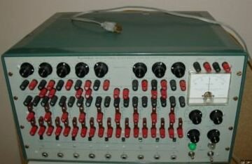
Figure 1 — A production-example Heathkit EC-1 in working order. The wrinkle-finish steel cabinet, aluminum front panel, and glowing tube complement are visible. The patch board occupies the upper left quadrant; balance pots line the bottom rail.

About This Volume

Volume 1 establishes the historical, conceptual, and physical foundation for the entire series. It answers three questions a senior engineer would ask before spending time on an unfamiliar machine: What is it, exactly? Why does it matter? Is mine worth restoring? Technical depth increases sharply in the volumes that follow; this volume deliberately keeps circuit equations at the survey level so that the architecture discussion in Section 2 is accessible before the reader has studied the schematics.

Depth-Index: The Eight-Volume Series

Vol	Title	Primary Content
1	Overview & History (this volume)	Historical context, physical tour, specifications quick-table, acquisition decision tree
2	Hardware & Theory of Operation	6U8 triode-pentode topology, gain derivation (~1 000 open-loop), virtual-ground analysis, NE-2H neon level-shift, power supply architecture
3	Patch Panel & Computing Elements	Patch-board socket map, jack/pot reference table, computing element configurations, sign-convention discipline
4	Acquisition & Restoration	Safety protocol, variac soak, full BOM with Digi-Key part numbers, capacitor reforming vs. replacement, selenium-rectifier substitution
5	Programming	Scaling methodology, RC time-constant selection, block-diagram to patch translation, ODE setup
6	Sample Programs & Demonstrations	Falling body, spring-mass SHM, damped oscillator, projectile with drag, logistic growth, predator-prey
7	Modern Extensions & Interfacing	Solid-state substitution, data-logging, ±60 V → ±5 V attenuator board, Arduino/Raspberry Pi ADC interface
8	Cheatsheet	Field-grade quick-reference: tube map, jack/pot map, scaling formulas, patch symbols, power-up sequence

Note — Cross-references appear throughout as “see Vol N §M.” All volume text is self-contained; Vol 1 does not assume the reader has read any other volume.

What the EC-1 Is

Analog vs. Digital Computation

A digital computer encodes every quantity as a binary integer, processes it through clocked logic gates, and approximates continuous-time phenomena by iterating a discrete numerical algorithm. An analog computer encodes quantities as instantaneous voltage levels and processes them by exploiting the physical laws of passive and active circuit elements. Integration is not approximated by a Euler step — it is performed by a capacitor charging through a resistor, exactly and continuously, as fast as the circuit time constant allows.

The distinction has engineering consequences that remain relevant for study today:

Property	EC-1 (analog)	Digital computer
Variable representation	Continuous voltage (±60 V full scale)	Discrete integer (fixed or float)
Integration	Physical RC: exact in real time	Numerical method (Euler, RK4, etc.)
Parallelism	All nine op-amps run simultaneously	Serial or pipelined; no inherent parallelism
Accuracy	~1 % (resistor + amp tolerances)	Governed by word length; fp32 ~7 decimal digits
Reprogramming	Rewire; seconds to minutes	Reload; microseconds
Parameter sensitivity	Turn a knob; see result in real time	Re-run simulation after each parameter change
Noise amplification	Differentiation avoided; integration preferred	Not a hardware constraint

The EC-1 can solve any ordinary differential equation (ODE) expressible in terms of addition, multiplication by a constant, and integration. Shannon (1941) proved this is sufficient to compute any continuous function. Non-linear operations — saturation, hysteresis, limit stops, diode rectification — are added by inserting crystal diodes and relay contacts into the patch network.

Voltage Convention and Scale Factors

The EC-1 represents a problem variable u as a voltage e related by an amplitude scale factor a:

e = a · u

The output rail of each operational amplifier is rated at ±60 V at 0.7 mA continuous. The operator chooses a so that the expected maximum of u maps to no more than ±60 V — typically ±50 V to leave headroom. If a variable ranges 0–100 m/s, setting a = 0.5 V/(m/s) maps the range to 0–50 V. After computation, output voltages are divided by a to recover physical values.

A second scale factor governs time. When the input resistor Rᵢ = 1 MΩ and the feedback capacitor Cᶠ = 1 µF, the integrator time constant τ = Rᵢ Cᶠ = 1 s, and computation proceeds in real time. Substituting Rᵢ = 0.1 MΩ compresses the time axis by 10×, solving the same ODE ten times faster — essential when the physical phenomenon takes minutes but the repetitive oscillator needs to cycle at several hertz for oscilloscope display.

Real-Time Circuit Mathematics

The diagram below shows the four canonical op-amp configurations produced by patch-cord and plug-in selection. Every problem on the EC-1 is assembled from these building blocks (see Vol 5 for detailed setup procedures).

┌─────────────────────────────────────────────────────────────────────────┐
│   INVERTER / SCALER           SUMMER                                    │
│                                                                         │
│   e₁ ──[Rᵢ]──┬──[Rf]──┐   e₁ ──[R₁]──┐                               │
│               ↓   ┌─►──┤   e₂ ──[R₂]──┼──[Rf]──┐                     │
│              [A]──┘    │               ↓   ┌─►──┤                     │
│               │        │              [A]──┘    │                      │
│              eₒ = -(Rf/Rᵢ)·e₁        │        eₒ = -(Rf/R₁·e₁        │
│                                       │              + Rf/R₂·e₂ + …)   │
│                                      eₒ                                │
│                                                                         │
│   INTEGRATOR                          COEFFICIENT POT                  │
│                                                                         │
│   e₁ ──[Rᵢ]──┬──[Cf]──┐             Vref ──┤POT├──► eₒ = k·Vref      │
│               ↓   ┌─►──┤             (k set 0–1 by front-panel knob)  │
│              [A]──┘    │                                               │
│               │        │                                               │
│     eₒ = -(1/RᵢCf)∫e₁ dt                                              │
└─────────────────────────────────────────────────────────────────────────┘
  [A] = inverting high-gain amplifier (one 6U8 tube each, gain ≈ 1 000)
  Standard values: Rf = Rᵢ = 1 MΩ; Cf = 1 µF → τ = 1 s (real time)

Note — The EC-1’s op-amps are inverting, so every stage contributes a sign change. The programmer must track polarity through the signal chain and insert an extra inverter wherever a positive quantity is required. The operational manual conventions are covered in Vol 6; the hardware reality of why the gain is −1 000 (not +1 000) is derived in Vol 2.

Historical Context, 1959–1971

The Analog Era and Its Practitioners

From approximately 1945 to 1965 the vacuum-tube analog computer was the dominant tool for continuous-system simulation in aerospace, ordnance, and process engineering. REAC (Reeves Electronic Analog Computer, 1947), the Goodyear GEDA, Beckman EASE, and Philbrick K2-W-based desk-top units were the professional-grade machines. A complete installation occupied a room and cost $50 000 to $500 000 (1955 dollars). The mathematics being solved — ballistic trajectories, control-loop transients, structural dynamics — were identical to what engineers write down today; the difference was the hardware.

Heath Company and the EC-1

The Heath Company of Benton Harbor, Michigan, introduced the EC-1 Educational Analog Computer in 1959 (preliminary design dated 3/20/59 per the operational manual preface). The machine was sold until approximately 1971 — a twelve-year production run that coincides almost exactly with the Apollo programme. It was available in two forms:

Form	Price
Kit (self-assembly)	$199.95
Factory-assembled	~$400

The kit price was strikingly low. Contemporary professional machines cost thousands of dollars for a single operational amplifier module; the EC-1 delivered nine complete amplifiers plus power supplies, patching hardware, and documentation for less than a week’s median engineering salary. This positioning was deliberate: Heathkit’s business model, established with amateur radio gear and test equipment, was to democratize technology through well-documented kits. The EC-1 extended that philosophy into computation.

Adoption was rapid across two communities:

Industry: Engineering departments at aerospace contractors, automotive companies, and chemical plants used the EC-1 to train analog computer operators and to prototype problem setups before committing machine time on larger installations.
Academia: Universities and secondary schools acquired the EC-1 to teach control theory, differential equations, and physical simulation. The operational manual’s reference list cites Korn & Korn (Electronic Analog Computers, McGraw-Hill, 1956) and Clarence L. Johnson (Analog Computer Techniques, McGraw-Hill, 1956) — the canonical graduate-level texts — indicating that Heath positioned the EC-1 as a gateway to professional practice, not a toy.

Displacement by Digital Computation

The transition away from analog computing began in earnest around 1965 with the availability of transistorized minicomputers (DEC PDP-8, 1965; IBM System/360, 1964). Digital machines offered higher accuracy, non-volatile program storage, and the ability to solve non-continuous problems (combinatorial logic, sorting, text processing) that analog hardware cannot address. By 1971, when Heath discontinued the EC-1, integrated-circuit operational amplifiers (the µA741 was introduced in 1968) had already made the vacuum-tube analog op-amp obsolete for new designs.

The EC-1 nonetheless remains historically important for three reasons:

Pedagogical clarity. The physics of integration, scaling, and sign convention are visible in the wiring. A student who patches a spring-mass oscillator and watches the sine wave appear on an oscilloscope has direct kinesthetic understanding of what numerical integration is approximating.
Real-time continuous simulation. The machine solves its ODE in hardware-parallel real time, a property no digital computer achieves for general ODEs without dedicated FPGA or analog-front-end hardware.
Historical artifact. The EC-1 was contemporary with early Atlas, Mercury, and Gemini simulation work. The identical mathematical apparatus — two integrators plus an inverter plus a coefficient pot — that produces a mass-spring simulation on the EC-1 was the basis for real missile trajectory calculations of that era.

Timeline Summary

Year	Event
1947	REAC introduced; analog computing enters industrial use
1956	Korn & Korn textbook defines professional analog computer practice
1959	Heath Company introduces EC-1; price $199.95 kit
1960–65	Peak academic and industrial adoption; Apollo-era simulation programs
1964–65	IBM 360 / DEC PDP-8 shift professional market toward digital
1968	Fairchild µA741 IC op-amp; vacuum-tube analog amps commercially obsolete
1971	EC-1 production ends; approximately 12-year run
2016	Nuts & Volts restoration article re-introduces the EC-1 to makers
2024–26	Active collector/restoration community; working units appear at hamfests and eBay

Physical Tour

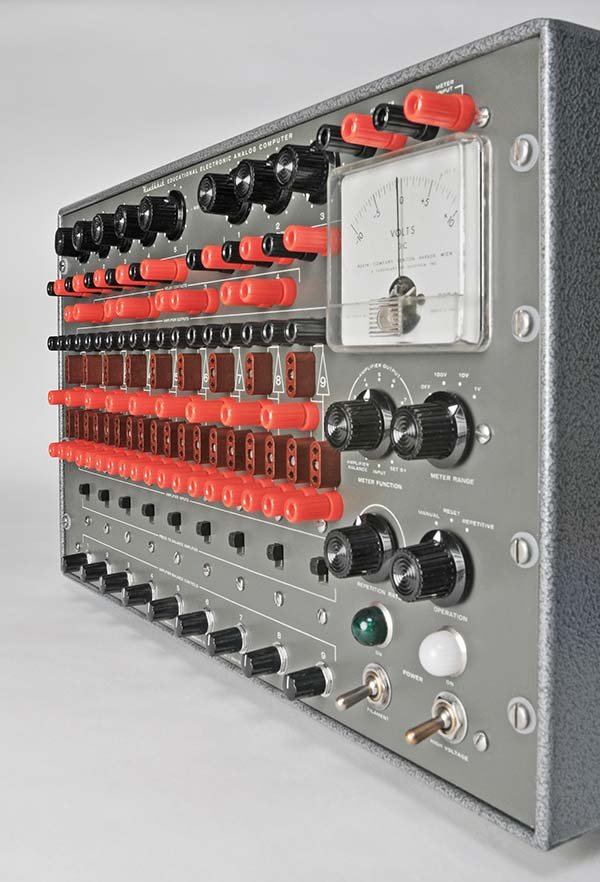
EC-1 front panel after restoration, showing patch board, balance pots, and meter.

Figure 2 — Restored front panel. The 27 two-pin patch sockets occupy the upper section; nine amplifier balance pots line the bottom rail; the 50-0-50 µA meter and function-select switches are visible in the center-right area.

Cabinet and Overall Dimensions

The EC-1 is housed in a steel cabinet with gray wrinkle-finish paint, a heat-activated crinkle lacquer that was standard on laboratory instrumentation of the period. The aluminum front panel is silk-screened in white. Dimensions and mass:

Dimension	Value
Width	19¾ in (501 mm)
Height	11½ in (292 mm)
Depth	15 in (381 mm)
Shipping weight	~43 lb (~19.5 kg)

The chassis is a conventional chassis-and-deck construction: a steel outer shell encloses a removable aluminum chassis plate on which the tube sockets, transformers, and terminal strips are mounted. The front panel is a separate piece bolted to the chassis with perimeter screws. Five parallel bus bars run the length of the chassis interior distributing +300 VDC, −150 VDC, and 6.3 VAC heater current to all nine amplifier tube sockets.

Danger — Internal voltages reach +300 V DC and −150 V DC. The filter capacitors hold lethal charge after power-off. Before touching any internal point, confirm with a meter that all capacitors have discharged. See Vol 4 §2 for the full lock-out/tag-out procedure.

Front Panel Layout — Functional Zones

The front panel divides into five functional zones described below. A complete jack-by-jack map appears in Vol 4.

┌───────────────────────────────────────────────────────────────────────────────┐
│  ZONE A: PATCH BOARD (upper left, ~60% of panel width)                       │
│  27 two-pin brown sockets for resistor / capacitor plug-in units             │
│  Arranged in a 3-row × 9-column array                                        │
│  Adjacent red (signal) and black (common) banana binding posts               │
│  for each amplifier I/O and IC supply output                                 │
├───────────────────────────────────────────────────────────────────────────────┤
│  ZONE B: COEFFICIENT POTS (upper right, 5 pots)                              │
│  5 × panel-mounted coefficient potentiometers                                │
│  One end grounded; wiper and high end brought to binding posts               │
│  Range: 0.000 to 1.000 (ratio of wiper voltage to end-to-end voltage)       │
├───────────────────────────────────────────────────────────────────────────────┤
│  ZONE C: METER / FUNCTION SELECTION (center right)                           │
│  50-0-50 µA D'Arsonval movement, 10 000 Ω/V sensitivity                     │
│  METER RANGE switch: 1 V / 10 V / 100 V / OFF                               │
│  METER FUNCTION switch: SET B+ / BALANCE / AMP 1–9 / INPUT                  │
│  AMPLIFIER OUTPUT binding posts: red+black, for external oscilloscope        │
│  METER INPUT binding posts: disconnects meter from computer for ext. use     │
├───────────────────────────────────────────────────────────────────────────────┤
│  ZONE D: MODE CONTROL (center right, below meter)                            │
│  OPERATION switch: RESET / MANUAL / REPETITIVE                               │
│  FILAMENT switch + green pilot lamp                                          │
│  HIGH VOLTAGE switch + clear pilot lamp                                      │
│  REPETITION RATE control: 0.1–15 cps (adjusts multivibrator period)         │
├───────────────────────────────────────────────────────────────────────────────┤
│  ZONE E: INITIAL CONDITION SUPPLIES (bottom right, 3 supplies)               │
│  IC-1, IC-2, IC-3: each 0–105 V output, max 5 mA, ungrounded               │
│  One panel pot per supply; red (+) and black (−) binding posts               │
│  Relay contacts: 4 sets (1–4) brought to binding posts for IC switching     │
├───────────────────────────────────────────────────────────────────────────────┤
│  ZONE F: AMPLIFIER BALANCE POTS (bottom rail, 9 pots)                       │
│  Nine 3 kΩ wire-wound pots (one per amplifier)                              │
│  Slide switch above each pot disconnects amplifier from patch board          │
│  during balancing, inserting standard 1 MΩ / 1 MΩ feedback network         │
└───────────────────────────────────────────────────────────────────────────────┘

Tube Complement

Nine identical operational amplifiers each use one 6U8 dual-triode/pentode. The pentode section provides the high-gain stage; the triode section drives the output cathode-follower. Two NE-2H neon lamps per amplifier serve as a voltage-level-shifting reference (see Vol 2 §3 for the circuit analysis).

Tube	Qty	Function	Notes
6U8	9	DC operational amplifier	Pentode gain stage + triode cathode follower
6AQ5	1	Power stage / relay driver	Output of repetitive oscillator
12BH7	1	Repetitive oscillator multivibrator	Sets 0.1–15 cps cycle rate
0A2	1	−150 V VR tube regulator	150 V regulation; purple/blue glow characteristic
0B2	1	IC supply VR tube regulator	108 V drop; same glow
6BH6	1	Meter / buffer function	Controls / read-out section

Tip — The OA2 and OB2 glow a distinctive violet-blue when conducting. A dim or absent glow indicates the tube is not regulating; the −150 V rail will rise above specification and amplifier balance will be unstable. Replace before further troubleshooting.

Interior Chassis View

The interior chassis (accessible by removing the front panel and lid) reveals the physical bus structure and component layout:

  TOP OF CHASSIS (looking down from above, lid removed)
  ┌─────────────────────────────────────────────────────────────┐
  │  POWER TRANSFORMER   FILTER CAPS   RECTIFIER STACK         │
  │  (rear left)         (rear center) OA2/OB2 VR tubes        │
  │                                    (rear right)             │
  ├─────────────────────────────────────────────────────────────┤
  │  ─── +300 V BUS ──────────────────────────────────────────  │
  │  ─── −150 V BUS ──────────────────────────────────────────  │
  │  ─── HEATER 6.3 VAC ──────────────────────────────────────  │
  │  ─── COMMON / SIGNAL GND ─────────────────────────────────  │
  │  ─── CHASSIS GND ─────────────────────────────────────────  │
  ├─────────────────────────────────────────────────────────────┤
  │  6U8 #1  6U8 #2  6U8 #3  6U8 #4  6U8 #5                   │
  │  (tube sockets in two rows)                                  │
  │  6U8 #6  6U8 #7  6U8 #8  6U8 #9  12BH7  6AQ5  6BH6       │
  ├─────────────────────────────────────────────────────────────┤
  │  RELAY (4PST, normally closed)   IC SUPPLY POTS (×3)       │
  │  TERMINAL STRIPS (patch connections)                         │
  └─────────────────────────────────────────────────────────────┘

The five bus bars run front-to-rear along the chassis deck, soldered to each tube socket at the appropriate pin. This architecture makes the EC-1 significantly easier to trace than a point-to-point wired instrument: any amplifier’s supply connections are on the same pins of every socket. See Vol 2 for power-supply detail and Vol 4 for chassis-disassembly procedure.

Decision Tree — Is the EC-1 the Right Machine?

The decision tree below helps an engineer or educator evaluate whether to acquire, restore, and operate an EC-1, or whether a different approach better serves the goal.

                    ┌─────────────────────────────────────────┐
                    │  What is the primary goal?              │
                    └──────────┬──────────────────────────────┘
                               │
           ┌───────────────────┼───────────────────┐
           ▼                   ▼                   ▼
   ┌───────────────┐   ┌───────────────┐   ┌───────────────┐
   │  Solve a real │   │  Teach analog │   │  Collect /    │
   │  engineering  │   │  computing    │   │  preserve     │
   │  ODE today    │   │  concepts     │   │  history      │
   └───────┬───────┘   └───────┬───────┘   └───────┬───────┘
           │                   │                   │
           ▼                   ▼                   ▼
   ┌───────────────┐   ┌───────────────┐   ┌───────────────┐
   │Need ≥1% acc.? │   │Hands-on demo? │   │EC-1 available?│
   └──┬────────┬───┘   └──┬────────┬───┘   └──┬────────┬───┘
      │YES     │NO        │YES     │NO         │YES     │NO
      ▼        ▼          ▼        ▼           ▼        ▼
  Use SPICE  EC-1 is  EC-1 is  Simulation  Restore   Consider
  or MATLAB  marginal; excellent  software   the unit  HP/EAI/
  for prod.  fine for   choice   (MATLAB,    (see      Philbrick
  work.      tutorial   ✓        QUCS) may   Vols 4–7) machines
             purposes.           suffice.              for
                                                       variety.

Key considerations at each branch:

Accuracy requirement. At ±1 % resistor tolerance and ~1 000 open-loop gain, amplifier error is on the order of 0.1–1 % per stage; chain errors accumulate. Problems requiring five or more cascaded operations may exhibit 3–5 % total error. For tutorial and demonstration purposes this is entirely acceptable; for production engineering it is not.
Teaching value. The EC-1’s primary modern value is pedagogical. The kinesthetic connection between patching a circuit, setting initial conditions, and watching a waveform emerge on an oscilloscope is not reproducible by any simulation package. If the goal is to make differential equations visceral, the EC-1 has no digital equivalent.
Condition assessment. Before committing to restoration, inspect for: (a) absent or shattered tubes — 6U8 availability is moderate, NOS units at approximately $5–15 each; (b) burned transformer — visible scorching or melted insulation; (c) corroded or broken front-panel silk screening — essentially irreplaceable; (d) missing two-pin plug-in hardware — machined replicas required. A unit with all tubes present and an intact front panel is a strong restoration candidate. See Vol 5 §1 for the full pre-restoration inspection checklist.
Secondary market pricing. Units appear on eBay at $420–$1 500 depending on condition. The 2016 Nuts & Volts restoration (Goodsell, May 2016) documented a purchase price of $420. Budget an additional $100–$300 for capacitors, balance pots, tube testing, and hardware.

Tip — Units described as “powers on” are not necessarily functional — tubes degrade, balance pots drift, and electrolytic capacitors dry out over 50+ years. A unit that powers on without smoke is merely a better starting point than one that does not, not a finished instrument.

Specifications Quick-Table

Electrical Specifications

Parameter	Value	Notes
Operational amplifiers	9	One 6U8 per amplifier
Open-loop voltage gain	~1 000	Pentode gain ~700; positive feedback raises to ~1 000
Output voltage range	±60 V	Rated; do not exceed ±60 V to protect NE-2H lamps
Output current	0.7 mA per amplifier	Cathode-follower output stage
Bandwidth (−1 dB)	600 Hz	Sufficient for mechanical simulation time-scaled to seconds
Input impedance	Very high (grid input)	1 MΩ resistors define effective input impedance in practice
Balance adjustment	3 kΩ wire-wound pot per amplifier	Zeroed in three successive passes: 100 V, 10 V, 1 V range

Power Supplies

Supply	Nominal	Regulation Method	Notes
+300 V (amplifier B+)	+300 VDC @ 25 mA	Electronic regulator (adjustable +250 to +350 V)	Set via VC pot on chassis and front-panel SET B+ position
−150 V (amplifier bias)	−150 VDC @ 40 mA	OA2 VR tube	Half-wave rectifier; purple glow indicates normal operation
IC supplies (×3)	0–105 V, ungrounded	OB2 VR tube + pot per supply	5 mA maximum; reversible polarity by binding-post selection
Heater	6.3 VAC	Transformer-secondary (unregulated)	All tubes; leave on ≥30 min before use
AC mains	105–125 VAC, 50/60 Hz	—	100 W total consumption

Patch and Control Hardware

Item	Quantity	Specification
Two-pin patch sockets	27	Brown bakelite; accept resistor/capacitor plug-in units
Amplifier input/output binding posts	18 red + 18 black	One pair input, one pair output per amplifier
Coefficient potentiometers	5	Panel-mounted, 0–1 range; wiper and ends at binding posts
Relay contacts	4 sets	4PST, normally closed; open in MANUAL/REPETITIVE
Initial condition controls	3	One pot each; 0–105 V output; max 5 mA
Repetitive oscillator range	0.1–15 cps	Multivibrator (12BH7); adjusted by panel control
Panel meter	50-0-50 µA	D’Arsonval movement; 10 000 Ω/V; three ranges
Amplifier output (external)	1 pair binding posts	Selects any of 9 amplifiers; connects to oscilloscope or recorder

Physical

Parameter	Value
Cabinet finish	Steel, gray wrinkle-finish (VHT-equivalent lacquer)
Front panel	Aluminum, white silk-screened legends
Width	19¾ in (501 mm)
Height	11½ in (292 mm)
Depth	15 in (381 mm)
Shipping weight	~43 lb (~19.5 kg)
Power consumption	100 W
Operating environment	Bench-top; no forced cooling required

Accuracy and Limitations

Source of Error	Magnitude	Mitigation
Resistor tolerance (supplied 1 % precision)	±1 % per element	Use 1 % or better; verify with 4-wire measurement
Amplifier finite gain (A ≈ 1 000)	~0.1 % per stage	Calibrate gain; acceptable for tutorial use
Amplifier drift (thermal)	Millivolt-level over minutes	Re-balance every 10–15 min during long runs
Capacitor leakage (feedback C)	Integrator error grows with run time	Limit runs to 1–5 min; see Vol 6 §4
Power supply variation	<1 % if VR tubes conducting	Verify OA2/OB2 glow before each session
Potentiometer resolution	Manual setting; ~0.5 % practical	10-turn pots (optional retrofit) improve coefficient precision

What Comes Next

Volume 1 has established the physical and historical context. The reader who continues into Vol 2 encounters the full circuit analysis of the 6U8 operational amplifier: pentode gain derivation, the role of the 2.2 MΩ positive-feedback resistor in extending gain to ~1 000, the virtual-ground approximation and its validity limits, the NE-2H neon level-shift network, and the power supply architecture. Vol 3 covers the patch panel, computing element configurations, and sign-convention discipline. Readers with a working machine who want to compute immediately should jump to Vol 5 (programming) and Vol 6 (sample programs), returning to Vols 2–4 when a circuit-level question arises.

Note — The Nuts & Volts (May 2016) restoration article by Goodsell is the most detailed first-person account of a complete EC-1 restoration in the public literature. It documents the $420 eBay acquisition, full disassembly and photograph protocol, electrolytic-capacitor replacement using modern parts slipped inside original paper sleeves, balance-pot replacement, and bouncing-ball demonstration setup. Summaries of its key findings appear throughout Vols 4 and 7.