Heathkit EC-1 · Volume 3
Heathkit EC-1 — Volume 3 — Patch panel & computing elements
Signal routing, op-amp configurations, and computing element reference — bridging Vol 2 power/hardware to Vol 4 problem scaling
3.1 About this Volume
Volume 3 covers the operating layer of the Heathkit EC-1: the patch panel through which the operator constructs every computation, and the four classes of computing element — the inverting summer, the integrator, the coefficient potentiometer, and the high-gain comparator — that collectively implement any ordinary differential equation solvable on the machine.
The treatment proceeds from the physical panel outward to the mathematics. Section 2 maps every jack, socket, bus, and binding post on the 19¾-inch panel. Sections 3 through 6 develop each computing element from first principles, grounding each in the specific EC-1 topology (6U8 tube, 1 MΩ feedback, ±60 V signal range). Section 7 closes with a fully worked single-element example — one integrator solving ẏ = −ky — that ties every prior concept together and sets up the multi-amplifier programs treated in Vol 4.
Scope and relationship to other volumes. Vol 2 covers the chassis hardware and power architecture (±300 V, −150 V, 6.3 VAC heaters, OA2/OB2 voltage regulators, and the three 100 V initial-condition supplies). Vol 4 covers acquisition and restoration procedures. Vol 5 covers amplitude and time scaling, multi-loop block diagrams, and the full programming methodology. Vol 6 covers sample programs. The present volume assumes the reader has already verified power supplies at the values given in Vol 2 and has balanced all nine amplifiers per the procedure summarised in Section 3.5 below.
Note — All voltages in this volume are referenced to the single machine ground (black binding posts). The EC-1 uses a single-ended, unipolar ground rail; the ±60 V signal range is ±60 V with respect to that rail, not a differential pair.
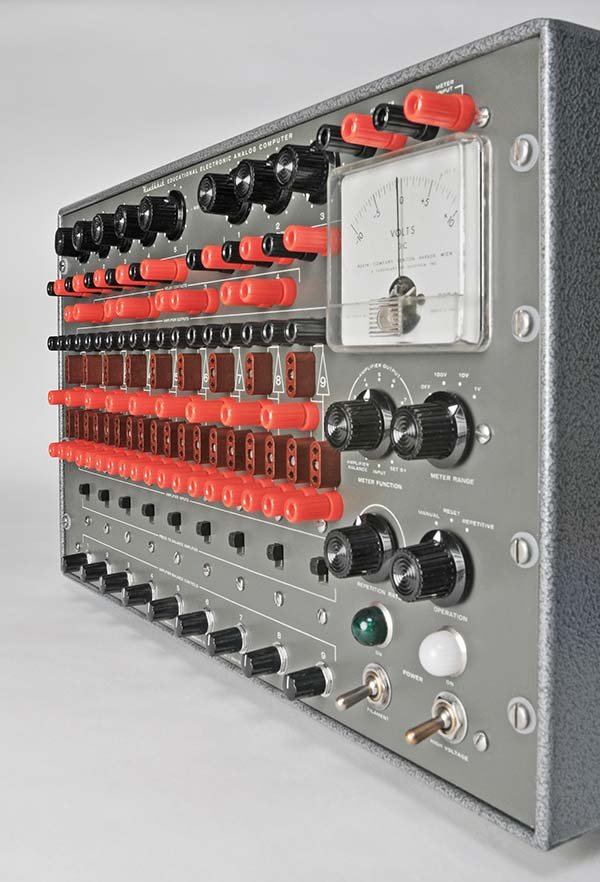
3.2 Patch-Panel Layout — Jacks, Buses, and Binding-Post Field
3.2.1 Physical organisation
The EC-1 front panel is a single anodised aluminium plate, 19¾” × 11½”, carrying all operator-accessible connections. The layout divides into six functional zones arranged in approximate rows from top-left to bottom-right:
Table 1 — The EC-1 front panel is a single anodised aluminium plate, 19¾" × 11½", carrying all operator-accessible connections. The layout divides into six functional zones arranged in approximate rows from top-left to bottom-right
| Zone | Location on panel | Contents |
|---|---|---|
| Amplifier modules 1–9 | Upper two-thirds, left to right | Two INPUT jacks + one FEEDBACK socket per amp; two OUTPUT jacks per amp; one BALANCE slide switch per amp |
| Patch-board sockets | Distributed among the amplifier modules | 27 two-pin brown sockets for plug-in resistors and capacitors |
| Coefficient potentiometers | Lower centre | 5 × 100 kΩ pots; each has a RED (high) and BLACK (wiper/ground) binding post |
| Initial condition supplies | Lower left | 3 × IC supplies, each with a RED (+) and BLACK (−) binding post and a rotary knob; output 0–100 V at 5 mA |
| Relay contacts | Lower left area | 4 sets of normally-closed SPST contacts brought to RED + BLACK binding posts for patch use |
| Meter and readout | Lower right | 50-0-50 µA meter; METER FUNCTION rotary (positions 1–9 = amplifier outputs, SET B+, INPUT, AMPLIFIER BALANCE); METER RANGE (1 V / 10 V / 100 V / OFF); AMPLIFIER OUTPUT binding posts (RED + BLACK); METER INPUT binding posts (RED + BLACK) |
The OPERATION switch (RESET / MANUAL / REPETITIVE) and REPETITION RATE control occupy the lower-right corner. The FILAMENT and HIGH VOLTAGE power switches are at the far right.
3.2.2 The patch-board socket grid
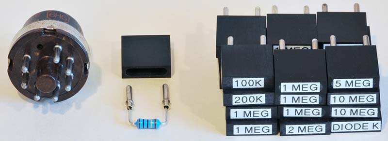
The 27 two-pin brown sockets are the key distinguishing feature of the EC-1 relative to professional machines that use fixed front-panel patch jacks. Each socket accepts a two-pin plastic plug on which a discrete resistor or capacitor is mounted. The two pins connect to the two binding posts that flank each socket on the panel: one post is connected to the amplifier summing junction (the virtual ground); the other connects to either an input drive point or the feedback return.
Note — The two-pin sockets are 0.300-inch centre-to-centre, matching the pin spacing of octal tube base pins. Operators who have exhausted the original plastic plugs can fabricate substitutes from octal base pins potted in Delrin rod stock (see Vol 4).
Each of the nine amplifiers has three sockets in a horizontal row:
  [ INPUT-A ]  [ INPUT-B ]  [ FEEDBACK ]
       |              |           |
   summing jct.   summing jct.  output node
The two input sockets share the same summing node; the feedback socket connects between output and summing junction. Placing a resistor in an input socket and a resistor in the feedback socket creates the summing configuration; placing a capacitor in the feedback socket creates the integrator.
3.2.3 Binding-post colour convention
Table 2 — Binding-post colour convention
| Colour | Meaning |
|---|---|
| Red | Signal-carrying or positive terminal |
| Black | Ground, return, or negative terminal |
The IC supply binding posts follow the same convention: RED = positive output terminal, BLACK = common (must be patched to machine ground before use, since the IC supplies are floating). The coefficient pot posts: RED = high end of the element (connected to the IC supply voltage), BLACK = wiper output.
3.2.4 Internal bus architecture
Five chassis-mounted bus bars distribute power to all nine amplifier sub-chassis:
Table 3 — Five chassis-mounted bus bars distribute power to all nine amplifier sub-chassis
| Bus | Voltage | Purpose |
|---|---|---|
| B+ | +300 VDC | Plate supply, regulated |
| B− | −150 VDC | Grid-bias / cathode supply, VR-tube regulated |
| Heater | 6.3 VAC | All tube heaters in series/parallel |
| IC common | Chassis GND | Reference for all signal voltages |
| Screen | Derived from B+ via resistor | 6U8 pentode screen at ~100 V |
These buses are internal and not operator-accessible; they appear on the schematic but not the patch panel. The operator interacts with the ±60 V signal domain exclusively through the front panel jacks.
Danger — The B+ bus operates at +300 VDC with respect to chassis. The chassis lid must be in place during operation. Do not probe internal buses with a voltmeter while the machine is powered unless using a meter rated for at least 500 V CAT I and taking the measurement from an isolated test point.
3.2.5 Jack and socket inventory
Table 4 — Jack and socket inventory
| Item | Qty | Panel label | Notes |
|---|---|---|---|
| Two-pin patch sockets | 27 | Unlabelled brown insert sockets | 3 per amplifier × 9 amps |
| Amplifier input binding posts | 18 | INPUT (per amplifier) | 2 per amplifier; share summing node |
| Amplifier output binding posts | 18 | OUTPUT (per amplifier) | 2 per amplifier; same node |
| Amplifier balance slide switches | 9 | (unlabelled, below each amp) | Disconnects amp from patch board during balance |
| IC supply binding posts | 6 | IC-1, IC-2, IC-3 (RED + BLACK each) | Floating supplies; ground one terminal |
| Relay contact binding posts | 8 | RELAY CONTACTS 1–4 (RED + BLACK each) | 4 × SPST, normally closed |
| Coefficient pot binding posts | 10 | POT 1–5 (RED + BLACK each) | 100 kΩ, one end grounded |
| Amplifier output readout posts | 2 | AMPLIFIER OUTPUT | RED + BLACK; connects to METER FUNCTION switch |
| Meter input posts | 2 | METER INPUT | RED + BLACK; isolated when FUNCTION ≠ INPUT |
3.3 Patch-Panel Signal-Flow Diagram
The following ASCII diagram represents the full front-panel connectivity for a typical three-amplifier configuration (two integrators plus one inverter), the minimum required to solve a second-order ODE. This layout also illustrates how the IC supplies, relay contacts, coefficient pot, and meter readout interact.
  ┌──────────────────────────────────────────────────────────────────────────────────────────┐
  │                         EC-1 FRONT PANEL — THREE-AMP LAYOUT                             │
  │                                                                                          │
  │  ┌────────────────────┐   ┌────────────────────┐   ┌────────────────────┐               │
  │  │  AMP 1 (Integrator)│   │  AMP 2 (Integrator)│   │  AMP 3 (Inverter)  │               │
  │  │  [IN-A][IN-B][FB ] │   │  [IN-A][IN-B][FB ] │   │  [IN-A][IN-B][FB ] │               │
  │  │   1MΩ        1µF  │   │   1MΩ        1µF  │   │   1MΩ        1MΩ  │               │
  │  │  INPUT ●  ● OUTPUT│   │  INPUT ●  ● OUTPUT│   │  INPUT ●  ● OUTPUT│               │
  │  │  [BAL slide sw]   │   │  [BAL slide sw]   │   │  [BAL slide sw]   │               │
  │  └────────┬───────┬──┘   └────────┬───────┬──┘   └────────┬───────┬──┘               │
  │           │ OUTPUT│               │ OUTPUT│               │ OUTPUT│                    │
  │           │       └───────────────►INPUT-A│               │       │                    │
  │           │               relay1  │       │   relay2       │       │                    │
  │  IC-1 RED►│INPUT-A  ●───────────►│       │◄─────────●────►│INPUT-A│                    │
  │           │ (RESET)   contacts    │       │ contacts       │       │                    │
  │           │                       │       │               │       │                    │
  │  ┌───────────────────────────────────┐    │      OUTPUT of Amp3 feeds back to           │
  │  │  RELAY CONTACTS 1 (NC=RESET)     │    │      Amp1 INPUT-B via Coeff Pot 1           │
  │  │  RED ●─────────────────────● BLK │    │                                            │
  │  └───────────────────────────────────┘    │                                            │
  │                                           │                                            │
  │  ┌──────────────────────────────────────────────────────────────────────┐               │
  │  │  COEFFICIENT POTS 1–5                                                │               │
  │  │  POT 1: RED ●──────[100kΩ]──────● BLACK(wiper)                      │               │
  │  │         (HIGH END: driven by Amp3 output or IC supply)               │               │
  │  │         (WIPER: patched to Amp1 INPUT-B or Amp2 INPUT-B)             │               │
  │  └──────────────────────────────────────────────────────────────────────┘               │
  │                                                                                          │
  │  ┌─────────────────────┐   ┌───────────────────────────────────────────────────────┐    │
  │  │  IC SUPPLIES 1–3    │   │  METER / READOUT                                      │    │
  │  │  IC-1: ●RED  ●BLK  │   │  FUNCTION: [1][2]...[9] [SET B+][INPUT][BAL]          │    │
  │  │  IC-2: ●RED  ●BLK  │   │  RANGE:    [1V][10V][100V][OFF]                       │    │
  │  │  IC-3: ●RED  ●BLK  │   │  AMP OUTPUT: ●RED  ●BLK                               │    │
  │  │  (0–100V, 5mA each)│   │  METER INPUT: ●RED  ●BLK                              │    │
  │  └─────────────────────┘   └───────────────────────────────────────────────────────┘    │
  │                                                                                          │
  │  OPERATION:  [RESET] [MANUAL] [REPETITIVE]        REP.RATE: ────────────[knob]          │
  └──────────────────────────────────────────────────────────────────────────────────────────┘

  Signal voltages: ±60 V nominal; ±100 V absolute maximum. Machine GND = chassis.
  All patch cords: banana-plug, red and black, 4"–24" lengths.
3.4 The Summer — Inverting Tube Op-Amp Summation
3.4.1 Topology and gain derivation
Each of the nine EC-1 amplifiers is a high-gain, DC-coupled, negative-feedback operational amplifier built around a single 6U8 dual-section tube. The 6U8 contains a pentode and a triode in one envelope; the pentode serves as the gain stage and the triode as a cathode-follower output buffer.
The virtual-ground (summing junction) analysis applies directly. With open-loop gain A ≈ 1,000 and maximum output ±60 V, the summing-junction voltage equals eₒ/A ≈ ±60 mV in the worst case — acceptably close to true virtual ground for a machine whose full-scale signal is ±60 V (0.1% error from this source alone).
The governing equation for n inputs is:
         Rf          Rf          Rf
eₒ = − ──── e₁  −  ──── e₂  − … ──── eₙ
         R1          R2          Rn
With R1 = R2 = … = Rn = Rf = 1 MΩ (the standard EC-1 precision resistors), this reduces to:
eₒ = −(e₁ + e₂ + … + eₙ)3.4.2 Gain selection by resistor ratio
The EC-1 operation manual (Ver 1, p. 5) specifies: “Generally, Rf is kept at 1 megohm and Ri is changed.” The practical gain range is 1 to 100; gains below unity tend toward instability in the 6U8 topology, and gains above 100 introduce unacceptable output error from summing-junction leakage.
Table 5 — Gain selection by resistor ratio
| Input resistor Ri | Feedback Rf | Gain magnitude |
|---|---|---|
| 1 MΩ | 1 MΩ | 1 (unity inverter) |
| 100 kΩ | 1 MΩ | 10 |
| 10 kΩ | 1 MΩ | 100 (practical maximum) |
| 500 kΩ | 1 MΩ | 2 |
| 200 kΩ | 1 MΩ | 5 |
Note — The EC-1 parts kit ships 1 MΩ precision (1%) resistors as the standard element. 100 kΩ precision resistors are used for ×10 gains. Other values (10 kΩ, 200 kΩ, 500 kΩ, 2 MΩ, 5 MΩ, 10 MΩ) must be separately procured for specialised problems such as the bouncing-ball demonstration.
3.4.3 The 6U8 amplifier circuit in detail
The pentode section of the 6U8 operates in a “starved” (low-screen-voltage) regime that maximises voltage gain while keeping the plate current low enough to work with practical plate-load values. The design achieves approximately 700× gain from the pentode stage alone. A small positive-feedback network (a 2.2 MΩ resistor from plate to screen) boosts the total open-loop gain to approximately 1,000.
A 1 kΩ / 5,600 pF high-frequency filter in the plate circuit rolls off the response above a few hundred kilohertz to prevent self-oscillation — a precaution necessary because a 1 MΩ feedback resistor combined with stray capacitance at the summing node would otherwise create a phase-shift oscillator. The −1 dB bandwidth with feedback applied is 600 Hz, which is entirely adequate for the differential-equation simulations the machine is designed to run (typically 0.1–15 Hz, limited by the repetitive oscillator).
The triode section of the 6U8 is wired as a cathode follower. Two NE-2H neon lamps act as a level-shifting element, dropping the plate voltage from the ≈+112 V quiescent level down to the ±60 V output range without the gain loss a resistive voltage divider would introduce. This neon-lamp level shifter is a distinctive element of the EC-1 design.
Amplifier electrical summary:
Table 6 — Amplifier electrical summary:
| Parameter | Value | Source |
|---|---|---|
| Tube | 6U8 pentode + triode | One per amplifier |
| Open-loop voltage gain A | ~1,000 | Manual Ver 1, p. 13 |
| Full-scale output swing | ±60 V | Operational; ±100 V absolute max |
| Rated output current | 0.7 mA (manual p. 3) / 3 mA (manual spec p. 32) | Use 0.7 mA as safe operating point |
| −1 dB bandwidth (closed loop) | 600 Hz | Spec sheet |
| B+ supply | +300 VDC | Electronically regulated |
| B− supply | −150 VDC | OA2 VR-tube regulated |
| Balance pot | 3 kΩ wirewound | One per amplifier |
| Summing-junction error (worst case) | ≤0.1% of full scale at unity gain | Derived from A = 1,000 |
3.4.4 The 6U8 tube — pin assignment and internal topology
The 6U8 is a combined pentode-triode in a 9-pin miniature (Noval) envelope. The EC-1 uses both sections:
Table 7 — The 6U8 is a combined pentode-triode in a 9-pin miniature (Noval) envelope. The EC-1 uses both sections
| Pin | Section | Connection in EC-1 |
|---|---|---|
| 1 | Triode plate | Cathode follower output stage; drives NE-2H level shift and output binding posts |
| 2 | Triode grid | Connected to pentode plate via 2.2 MΩ positive-feedback resistor network |
| 3 | Triode cathode | Output through NE-2H neon lamps; emitter of cathode follower |
| 4 | Heater | 6.3 VAC from heater bus |
| 5 | Heater | 6.3 VAC return |
| 6 | Pentode plate | Large plate-load resistor to B+ (+300 V); also drives HF filter (1 kΩ + 5,600 pF) |
| 7 | Pentode grid 1 (control) | Connected to summing junction through balance network |
| 8 | Pentode cathode | Bypassed to ground (cathode resistor sets operating point) |
| 9 | Pentode grids 2 & 3 (screen + suppressor) | Screen at ~100 V (resistor from B+); suppressor to cathode |
The “starved screen” technique (low screen voltage ≈ 100 V versus the normal 150–200 V) reduces the transconductance of the pentode but dramatically increases the plate resistance, which in combination with a high plate-load resistor yields the ~700× pentode gain. This approach was documented in the trade press by George Kaufer (“How to Design Starved Amplifiers,” Tele-Tech, January 1955) and by Walter Volkers (“Ultra-High-Gain Direct-Coupled Amplifier Circuits,” IRE National Convention, 1950), both cited in the EC-1 operation manual.
6U8 operating point (nominal, within the EC-1 amplifier):
Table 8 — 6U8 operating point (nominal, within the EC-1 amplifier):
| Parameter | Approx. value | Notes |
|---|---|---|
| B+ (plate supply) | +300 V | Regulated supply |
| B− (bias supply) | −150 V | VR-tube regulated |
| Pentode plate voltage | ~+200 V quiescent | Depends on balance setting |
| Screen voltage | ~+100 V | Resistor divider from B+ |
| Pentode cathode current | ~2–3 mA | |
| Triode plate voltage | ~+112 V | Before NE-2H level shift |
| NE-2H neon voltage drop | ~55–60 V per lamp (×2) | Sets the ±60 V output reference level |
| Output quiescent voltage | 0 V ± balance residual | After balance adjustment |
| Heater power | 6.3 V × 450 mA = 2.8 W | Per tube; 9 tubes ≈ 25 W heater load |
3.4.5 Amplifier balance procedure
Before each problem run, every amplifier must be balanced (output nulled to 0 V with no input). The balance slide switch on the panel disconnects the amplifier from the patch board and connects it in the standard 1 MΩ / 1 MΩ configuration (Fig. 13 in the operation manual). The 3 kΩ balance pot adjusts the grid-bias network to drive the output to zero. The procedure is performed iteratively at METER RANGE settings of 100 V, 10 V, and finally 1 V, converging the null to within ±10 mV.
Tip — Amplifier drift after warm-up is the dominant error source in long integration runs. The manual recommends a minimum 30-minute filament warm-up before use; the balance should be re-checked immediately before any precision run exceeding ~30 seconds.
3.4.6 Gain accuracy and error accumulation
In a multi-amplifier chain, the summing-junction error from finite open-loop gain accumulates. For a chain of n amplifiers each with gain error ε ≈ 1/A ≈ 0.1%:
Total gain error ≈ n × ε (for small ε, cascaded)With 9 amplifiers all in series (worst case), the cumulative error approaches 0.9% — still within the ±1% tolerance of the precision input resistors. In practice, deep-feedback loops tend to cancel rather than accumulate errors, so the real-world accuracy of the EC-1 is limited primarily by component tolerances (±1% for the precision resistors) and capacitor leakage, not amplifier gain error.
The manual (Ver 1, p. 5) notes: “In practice, the gain of DC computer amplifiers will vary from approximately 1000 for repetitive computers to as high as 10⁶ for a large commercial installation.” This places the EC-1 at the low end of the professional range — entirely appropriate for educational and demonstration use, and adequate for any problem whose solution accuracy requirements do not exceed 1–2%.
3.4.7 Sign convention
Every EC-1 amplifier inverts. This is not incidental but fundamental: it is required by the negative-feedback topology. The consequence for the programmer is that every integrator and every summer produces an output of opposite sign to its mathematical result. Sign chains must be tracked explicitly in the block diagram. The usual remedy is to pass through an even number of amplifiers in any feedback loop — an odd number creates positive feedback and oscillation.
Sign-chain tracking table for common configurations:
Table 9 — Sign-chain tracking table for common configurations:
| Amplifier role | Input sign | Output sign | Net sign through element |
|---|---|---|---|
| Inverter (unity) | + | − | −1 |
| Summer (2 inputs, unity) | both + | − | −1 per input |
| Integrator (RC) | + | − | −∫ dt |
| Two cascaded inverters | + | + | +1 |
| Integrator + inverter | + | + | +∫ dt |
| Integrator × 2 (loop) | + | + | Correct sign for d²/dt² |
3.5 The Integrator — Capacitor Feedback, Initial Conditions, IC/OPERATE/HOLD Modes
3.5.1 Switching the feedback element
An integrator is created by replacing the feedback resistor with a capacitor. With input resistor Ri and feedback capacitor Cf, the classical op-amp integrator equation applies:
         1     t
eₒ(t) = ─── ∫  eᵢ(τ) dτ + eₒ(0)
        RiCf  0
where eₒ(0) is the voltage on the capacitor at the start of the integration interval (the initial condition). With Ri = 1 MΩ and Cf = 1 µF, the time constant τ = RiCf = 1 s, yielding real-time integration. The factor 1/RiCf is the integration rate coefficient.
Integration rate (machine time constant) for common component combinations:
Table 10 — Integration rate (machine time constant) for common component combinations:
| Ri | Cf | RiCf | Relative speed |
|---|---|---|---|
| 1 MΩ | 1 µF | 1.0 s | Real time |
| 1 MΩ | 0.1 µF | 0.1 s | 10× faster |
| 0.1 MΩ | 1 µF | 0.1 s | 10× faster |
| 0.1 MΩ | 0.1 µF | 0.01 s | 100× faster |
| 1 MΩ | 10 µF | 10 s | 10× slower |
Note — The manual (Ver 1, p. 10) recommends keeping problem run times under 1–5 minutes because longer runs accumulate drift error and capacitor self-discharge error. For long time-constant problems, reduce RiCf by time-scaling the problem (see Vol 4).
3.5.2 Initial condition injection
The three floating IC power supplies (each 0–100 V, 5 mA, OB2 VR-tube regulated) provide the initial values loaded onto integrator feedback capacitors at the start of each run. The supplies are ungrounded; the operator patches one terminal to machine ground and applies the desired voltage to the input node. This allows either polarity (+) or (−) to be set as an initial condition, simply by choosing which terminal to ground.
Setting procedure for a +30 V initial condition:
- Black (−) terminal of IC-1 → machine ground (black binding post of any convenient amp).
- Verify METER FUNCTION = INPUT and read the IC-1 output at METER INPUT posts.
- Rotate the IC-1 knob clockwise until the meter reads 30 V on the 100 V range.
- Patch the red (+) terminal of IC-1 to the input binding post of the integrator amplifier.
The RESET state (OPERATION switch in RESET) closes the 4PST relay. The closed contacts short the feedback capacitor to ground through the relay path, simultaneously discharging any residual charge (clearing the “memory” of the previous run) and connecting the IC supply through the input resistor to precharge the capacitor to the desired initial condition.
Note — The relay contacts are “normally closed.” In RESET, contacts are closed. In MANUAL or REPETITIVE (OPERATE), contacts are open. This is the opposite of the intuitive “normally open” relay convention and must be borne in mind when tracing the circuit.
3.5.3 The three operating modes
Table 11 — The three operating modes
| Mode | OPERATION switch | Relay contacts | Computation state |
|---|---|---|---|
| IC (Initial Condition / RESET) | RESET | Closed | Capacitors discharged; IC voltages applied; output held at eₒ(0) |
| OPERATE | MANUAL | Open | Integration proceeds; output evolves per the differential equation |
| HOLD | (Not a dedicated switch; achieved by returning to RESET before run completes) | Closed | Freezes output voltage by shorting capacitor at its current value |
Note — The EC-1 does not have a dedicated HOLD switch in the same sense as a professional Philbrick or EAI machine. The closest equivalent is returning the OPERATION switch to RESET during a run, which both shorts the capacitor (freezing the integrand) and re-applies the IC. For a true HOLD (freeze without IC reset), a separate relay contact must be patched manually across the capacitor with the IC disconnected — a non-standard configuration described in the Nuts & Volts restoration article.
3.5.4 Repetitive operation and oscilloscope synchronisation
With the OPERATION switch in REPETITIVE, the 12BH7-based multivibrator drives the 4PST relay, cycling continuously between IC (relay closed) and OPERATE (relay open) at a rate set by the REPETITION RATE control: approximately 0.1 to 15 cycles per second. This mode is intended for oscilloscope display: the problem is solved, reset, and re-solved many times per second, producing a stable trace on a DC oscilloscope connected to AMPLIFIER OUTPUT. The oscilloscope sweep is not from the scope’s internal timebase; it is derived from another EC-1 integrator (configured as a ramp generator) to ensure synchronisation.
Ramp sweep generator configuration (one EC-1 amplifier consumed):
  IC-N RED ──[1MΩ]──► [Integrator Amp N] ──► SCOPE X-AXIS INPUT
                           1µF cap (Cf)
                           Relay contacts across Cf (same relay = reset every cycle)
The IC supply voltage sets the sweep rate. A −10 V IC input through a 1 MΩ / 1 µF integrator produces a ramp that rises at +10 V/s, reaching +60 V in 6 seconds — suitable for slow problems. Replace Ri with 100 kΩ for a ×10-faster sweep.
Timing diagram for REPETITIVE mode:
RELAY:    ──┐   CLOSED   ┌────────────────┐   CLOSED   ┌──
            │(OPERATE)   │   (RESET/IC)   │(OPERATE)   │
TIME:       │────────────►                │────────────►
            │  T_solve   │     T_reset    │  T_solve   │
            │            │                │            │
OUTPUT:     │  e^(-kt)  ─►  precharge y₀  │ e^(-kt)  ──►
The reset interval T_reset must be long enough for the relay to fully close, the capacitor to discharge, and the IC supply to precharge the capacitor to y₀. In practice, the relay bounce settles in <1 ms and the RC time constant for IC charging (IC impedance ≈ 100 kΩ, Cf = 1 µF → τ = 0.1 s) means a minimum reset interval of 0.3–0.5 s is needed. The multivibrator timing is adjusted by the REPETITION RATE control, which varies the timing capacitor charge current via a potentiometer.
Note — The 12BH7 multivibrator that drives the relay uses the same 12BH7 type as the triode output stage in various Heathkit oscilloscope and audio amplifier kits of the era. The tube is widely available as NOS stock. The relay itself is a standard 4PST type rated for the EC-1’s supply voltages; relay coil current is provided by the 6AQ5 output tube, which acts as the relay driver stage.
3.5.5 Capacitor selection and error sources
The standard feedback capacitor supplied with the EC-1 is a 1 µF Mylar (polyester film) type rated at 630 V. Mylar was chosen for its low dielectric absorption (DA) — a critical parameter for integrators, because DA causes the capacitor’s charge to partially “return” after discharge, introducing an offset error at the start of the next run. Modern equivalents are polypropylene film capacitors, which exhibit even lower DA and are preferred in restoration. Electrolytic capacitors must not be used as integrating capacitors; their leakage current and DA are far too high.
Integrator error budget (typical, room temperature):
Table 12 — Integrator error budget (typical, room temperature):
| Error source | Magnitude | Mitigation |
|---|---|---|
| Amplifier offset drift | <1 mV/min after 30-min warm-up | Balance before each run; limit run time |
| Capacitor leakage | <0.1 µA at 60 V (Mylar) | Use film caps; avoid electrolytics |
| Capacitor dielectric absorption | <0.1% of previous charge | Use polypropylene film; adequate reset time |
| Resistor tolerance (1% precision) | ±1% of computed integral | Use supplied 1% resistors |
| Summing-junction error (finite gain) | <0.1% at unity gain | Inherent; increases with gain ratio |
3.6 Coefficient Potentiometers — Setting Gains 0–1, Loading, Calibration
3.6.1 Physical description
Five 100 kΩ linear-taper wire-wound potentiometers are mounted along the lower edge of the front panel. Each pot has three terminals, two of which are wired to binding posts on the panel:
Table 13 — Five 100 kΩ linear-taper wire-wound potentiometers are mounted along the lower edge of the front panel. Each pot has three terminals, two of which are wired to binding posts on the panel
| Binding post | Connection | Function |
|---|---|---|
| RED | High end of resistance element | Connect to IC supply or signal source |
| BLACK | Wiper (centre lug) | Output — patched to amplifier input |
| (Internal) | Low end of resistance element | Wired to machine ground on the panel |
With this arrangement, the wiper output voltage equals:
V_wiper = V_RED × (dial fraction)where dial fraction is 0 (full counterclockwise = wiper at ground) to 1 (full clockwise = wiper at RED terminal). The coefficient potentiometer thus implements the multiply-by-constant operation for any constant k in [0, 1].
Note — The EC-1 coefficient pots implement only the range [0, 1]. Gains greater than 1 must be realised using the resistor-ratio method at the amplifier input sockets (e.g., Ri = 100 kΩ, Rf = 1 MΩ gives gain = 10). Negative gains are obtained by preceding or following the pot with an inverter amplifier.
3.6.2 Loading effect analysis
The source impedance of the pot wiper depends on the wiper setting. At mid-scale, the Thevenin source impedance is:
R_Thevenin = (R_total/4) × 2 / (R_total/2 + R_total/2) = R_total / 4 = 25 kΩIn the worst case (mid-scale setting), the source impedance is 25 kΩ. When the wiper is patched to an amplifier input socket where a 1 MΩ resistor is installed, the load on the wiper is 1 MΩ to the virtual ground of the summing junction — a negligible load (25 kΩ / 1 MΩ ≈ 2.5% voltage divider error). However, if the wiper is also driving a second load (e.g., patched to two amplifier inputs simultaneously), the load drops to 500 kΩ, increasing the error to approximately 5%.
Tip — To eliminate pot loading in critical measurements, buffer the wiper through a unity-gain inverter (one amplifier with Ri = Rf = 1 MΩ). The inverter’s high input impedance (virtual-ground summing junction with 1 MΩ series resistor effectively isolates the pot) prevents loading. This does invert the sign; a second inverter restores it.
3.6.3 Setting and calibration
The five pots do not have calibrated dials. The procedure for setting a coefficient k is:
- Connect the IC supply (at a known voltage V, e.g., 10 V) to the RED terminal of the pot.
- Connect the BLACK (wiper) terminal to the METER INPUT binding posts.
- Set METER FUNCTION = INPUT; METER RANGE = 10 V.
- Rotate the pot until the meter reads k × V (e.g., for k = 0.38, read 3.8 V).
- Patch the wiper (BLACK) to the amplifier input.
For the bouncing-ball problem (see Vol 6), coefficients representing gravity (g ≈ 9.8 m/s²), damping, and bounce restitution must all be set this way. It is good practice to measure each coefficient before a run and record it in the problem notebook.
Pot specification summary:
Table 14 — Pot specification summary:
| Parameter | Value |
|---|---|
| Total resistance | 100 kΩ |
| Taper | Linear |
| Construction | Wire-wound |
| Ground end | Internal, panel-wired to machine GND |
| Wiper output range | 0 V to V_RED |
| Maximum wiper current | 5 mA (IC supply rated at 5 mA; limit source current) |
| Mid-scale Thevenin impedance | 25 kΩ |
| Recommended load (no buffer) | ≥ 500 kΩ (i.e., ≥ one 500 kΩ input resistor) |
3.7 Sign Inversion and the High-Gain Comparator
3.7.1 Unity-gain inverter
Because every EC-1 amplifier is inherently inverting, a unity-gain inverter is simply an amplifier configured with Ri = Rf = 1 MΩ and no other inputs. This is the most common single-amplifier “helper” configuration in EC-1 programs:
  eᵢ ──[1MΩ]──► Σ ──► [A≈1000] ──► eₒ = −eᵢ
                 ↑_______[1MΩ fb]___|
Inserting an inverter after an integrator restores the expected sign; inserting one anywhere in a feedback loop changes the loop sign. The block diagrams in the operation manual show explicit triangular amplifier symbols but do not always label the inversions; the programmer must track signs manually.
3.7.2 Gain-of-ten scaler (sign-inverting)
A common variant is the ×10 inverting amplifier:
  eᵢ ──[100kΩ]──► Σ ──► [A≈1000] ──► eₒ = −10 eᵢ
                   ↑_______[1MΩ fb]___|
This is useful for amplitude unscaling: if the problem was scaled down by 10× to keep signals within ±60 V, the scaler restores the display-level output to a readable range before connecting to the meter or oscilloscope.
3.7.3 The high-gain comparator
When an EC-1 amplifier is operated without feedback (or with a very high impedance feedback element), its open-loop gain of ~1,000 causes the output to saturate — to rail at approximately +60 V or −60 V — for any non-zero differential input. This saturating behaviour is exploited as a comparator in the bouncing-ball problem: a diode and resistor network feeds the comparator input with the sum (ball height + threshold voltage). When height > 0, the comparator output is one polarity; when height < 0 (ball below floor), the output flips, driving a relay or switching circuit that reverses the velocity sign.
The EC-1 does not have a dedicated comparator module; the comparator function is realised by one of the nine general-purpose amplifiers configured in open loop or with a large-valued feedback resistor (10 MΩ is used in the bouncing-ball circuit described in the Nuts & Volts article). The two silicon diodes (1N4006 per the parts list) implement the nonlinear switching function:
Diode clamp: output of comparator ──[D1]──► velocity-reversal summing node
             Inverted output      ──[D2]──► (inactive path)
When the “floor contact” condition is satisfied, the diode conducts and injects a velocity-reversal signal. The result is a physically realistic bounce with energy loss set by the damping coefficient pot.
Note — The EC-1’s diode-comparator approach is a simplified analogue of the relay-switched “bounce” logic used in larger professional machines (EAI TR-48, Philbrick Computational Handbook setups). It introduces a small dead-band around the zero-crossing determined by the diode forward voltage (~0.6 V at operating current) and the amplifier gain, which is acceptable for demonstration purposes.
Summary: EC-1 amplifier configurations
Table 15 — Summary: EC-1 amplifier configurations
| Configuration | Input socket | Feedback socket | Gain characteristic | Output sign |
|---|---|---|---|---|
| Unity inverter | 1 MΩ | 1 MΩ | −1 | Inverted |
| Summer (2 inputs, unity) | 2 × 1 MΩ | 1 MΩ | −1 per input | Inverted sum |
| Scaler ×10 | 100 kΩ | 1 MΩ | −10 | Inverted, scaled |
| Scaler ×2 | 500 kΩ | 1 MΩ | −2 | Inverted, scaled |
| Integrator (real time) | 1 MΩ | 1 µF cap | −1/s (1/τ) | Inverted integral |
| Integrator (10× fast) | 100 kΩ | 1 µF cap | −10/s | Inverted integral |
| Open-loop comparator | 1 MΩ | None / 10 MΩ | ~±1000 (saturating) | Polarity of input |
3.8 Worked Single-Element Example — One Integrator Solving ẏ = −ky
3.8.1 Problem statement
Solve the first-order linear ODE:
dy/dt = −k y, y(0) = y₀This describes radioactive decay, RC circuit discharge, Newton’s law of cooling, and exponential population decay, depending on the physical interpretation. The analytic solution is y(t) = y₀ exp(−kt), a decaying exponential.
3.8.2 Machine equation formulation
The standard EC-1 programming approach starts from the highest-order derivative and integrates downward. Here:
ẏ = −k yRearranging for the integrator input:
integrator input = ẏ = −k y = −k × (output of integrator)The integrator output IS y; its input must receive ẏ. Substituting:
integrator input = −k × yBut the EC-1 integrator is inverting: eₒ = −(1/τ) ∫ eᵢ dt. So the output is −∫(input) dt. To make the output equal to y, the input must be set to ẏ with the sign reversed by the integrating inversion:
y = −(1/τ) ∫ (input) dtIf input = +k × y, then:
y = −(1/τ) ∫ k y dt → dy/dt = −(k/τ) yWith τ = 1 (Ri = 1 MΩ, Cf = 1 µF), this gives dy/dt = −k y as required. The coefficient pot sets k.
3.8.3 Block diagram
┌────────────────────────────────────────────────────────────┐
│                                                            │
│  IC supply ──► [Amp 1, integrator]  ──►  y(t) = y₀ e^-kt │
│                       ▲                          │        │
│                       │                          │        │
│              [Coeff Pot, set to k] ◄─────────────┘        │
│                                                            │
│  Patch: Pot-RED = IC-1; Pot-BLACK = Amp1 input socket      │
│         Amp1 feedback = 1µF cap; Relay contacts across cap  │
│         IC-1 (+) = y₀ voltage                              │
└────────────────────────────────────────────────────────────┘3.8.4 Patch-cord list
Table 16 — Patch-cord list
| From | To | Component in socket | Purpose |
|---|---|---|---|
| IC-1 RED | Pot 1 RED | — | Provides y₀ as the pot high-end voltage |
| IC-1 BLACK | Machine GND (any black post) | — | Grounds the floating IC supply |
| Pot 1 BLACK (wiper) | Amp 1 INPUT-A binding post | — | Delivers k·y to summing junction |
| Amp 1 OUTPUT RED | Pot 1 RED | — | Closes the feedback loop |
| Amp 1 INPUT-A socket | Two-pin plug | 1 MΩ precision resistor | Sets Ri |
| Amp 1 FEEDBACK socket | Two-pin plug | 1 µF Mylar 630 V capacitor | Sets Cf |
| Amp 1 INPUT binding post | Relay contacts 1 RED | — | Connects relay to reset cap |
| Amp 1 OUTPUT binding post | Relay contacts 1 BLACK | — | Other side of relay reset path |
| Amp 1 OUTPUT RED | AMPLIFIER OUTPUT RED | — | Readout to meter or scope |
Note — The pot RED terminal is driven by the output of Amp 1 during OPERATE mode and by the IC supply during RESET mode. A patch cord must connect both IC-1 RED and Amp 1 OUTPUT to the pot RED terminal simultaneously, relying on the fact that during RESET the amplifier output is held near y₀ by the IC precharge, and during OPERATE the IC supply current is too small to perturb the feedback. In practice, some operators disconnect the IC-1 lead from the pot RED terminal at the start of OPERATE for cleaner operation (using a third patch cord switched by hand or by routing through a relay contact).
3.8.5 Step-by-step operating procedure
- Power on — Filament switch ON; wait 30 minutes.
- Set B+ — METER FUNCTION = SET B+; adjust VC trimmer on chassis until meter reads the SET B+ mark (+300 V on the 100 V range).
- Balance Amp 1 — OPERATION switch = RESET. Depress Amp 1 balance slide switch. METER FUNCTION = AMPLIFIER BALANCE. Set RANGE = 100 V, then 10 V, then 1 V, adjusting the 3 kΩ balance pot each time until the meter reads zero.
- Set initial condition — Connect IC-1 BLACK to machine GND. Connect IC-1 RED and Amp 1 OUTPUT RED to METER INPUT posts (observe IC-1 voltage). Rotate IC-1 knob until meter reads y₀ (e.g., 30 V for y₀ = 30 V). Disconnect METER INPUT.
- Set coefficient — Connect IC-1 RED to pot 1 RED. Connect pot 1 BLACK (wiper) to METER INPUT RED. Set RANGE = 10 V. Rotate pot 1 until meter reads k × V_IC1 (e.g., k = 0.3: read 9.0 V). Disconnect METER INPUT.
- Patch the circuit — as per the patch-cord list above.
- OPERATE — Set OPERATION = MANUAL. The meter (FUNCTION = AMP OUT 1, RANGE = 100 V) should deflect rightward (positive) and decay exponentially. Time constant τ = 1/k seconds (k = 0.3 → τ ≈ 3.3 s at real-time scaling with Ri = 1 MΩ, Cf = 1 µF).
- Observe — On an oscilloscope: connect AMPLIFIER OUTPUT RED to scope channel, set to 20 V/div, DC coupled. Select REPETITIVE. Adjust REPETITION RATE so the trace just completes the decay before reset.
- RESET — OPERATION = RESET. Relay closes, capacitor discharges, IC precharge restores eₒ(0) = y₀.
3.8.6 Expected results and verification
At k = 0.3, y₀ = 30 V, Ri = 1 MΩ, Cf = 1 µF:
Table 17 — At k = 0.3, y₀ = 30 V, Ri = 1 MΩ, Cf = 1 µF:
| Time (s) | y(t) analytic | y(t) expected on meter |
|---|---|---|
| 0 | 30.0 V | 30 V (IC set) |
| 1 | 22.2 V | ~22 V |
| 2 | 16.4 V | ~16 V |
| 3 | 12.1 V | ~12 V |
| 5 | 6.7 V | ~7 V |
| 10 | 1.5 V | ~1.5 V |
The pot is set to k = 0.3 with the pot RED terminal at 30 V; the wiper delivers 9.0 V to Amp 1’s input. With Ri = 1 MΩ and Cf = 1 µF, the amplifier input current at t = 0 is 9 µA, and the initial rate of change is −9 V/s — consistent with ẏ(0) = −k y₀ = −0.3 × 30 = −9 V/s. This serves as the primary sanity check.
Tip — If the output stays flat (does not decay), check that the relay contacts are wired correctly and that the OPERATION switch is in MANUAL (not RESET, which keeps the contacts closed and prevents integration). If the output runs away to −60 V, the feedback loop sign is wrong — the pot is driving positive feedback. Verify that the output feeds the pot RED terminal (not a summing node directly) and that the pot wiper connects to the INPUT, not the FEEDBACK socket.
3.8.7 Scaling for a different time constant
To solve y(t) = 30 exp(−0.003 t) (i.e., k = 0.003 s⁻¹, time constant 333 s — suitable for simulating a thermal decay or slow chemistry), direct real-time computation would require 333 seconds of integration, accumulating excessive drift. The remedy is time-scaling by a factor of 100: replace Cf = 1 µF with Cf = 0.01 µF (or replace Ri = 1 MΩ with Ri = 10 kΩ), making the machine run 100× faster. Machine time τ_machine = 3.33 s; physical time τ_real = 333 s. Set the repetition rate accordingly. See Vol 4 for the complete time- and amplitude-scaling methodology.
3.8.8 Extension to second-order: the canonical loop
The single-integrator example scales directly to a second-order system by inserting a second integrator and an inverter (to manage sign). The canonical loop for ÿ + 2ζωₙ ẏ + ωₙ² y = 0 uses three amplifiers:
  ┌──── [Amp A: 1/s integrator] ─── ẏ ──── [Amp B: 1/s integrator] ─── y ────┐
  │                                                                             │
  │◄─── [2ζωₙ coefficient pot] ◄────────────────────────────────────────────────┤
  │◄─── [ωₙ² coefficient pot]  ◄──── [Amp C: inverter] ◄──────────────────────-┘
  │
  └──── Input of Amp A (ÿ = −2ζωₙ ẏ − ωₙ² y)
With ωₙ = 1 rad/s and ζ = 0.5 (underdamped), set the ωₙ² pot to 1.0 × (10 V reference) = 10 V, and the 2ζωₙ pot to 1.0 × (10 V) = 10 V, then scale to the ±60 V machine range by appropriate IC settings. The output y(t) is a damped sinusoid visible on the oscilloscope in repetitive mode — the classic spring-mass damping demonstration described in Vol 4, Section 2.
3.9 Machine Computing Capacity and Resource Allocation
3.9.1 Available computing resources
The EC-1’s total programming resources, understood as a budget the programmer must allocate across each problem, are:
Table 18 — The EC-1's total programming resources, understood as a budget the programmer must allocate across each problem, are
| Resource | Total available | Consumed per use | Notes |
|---|---|---|---|
| Operational amplifiers | 9 | 1 per function | Shared pool; any amp can be any function |
| Integrators | up to 9 | 1 amp + 1 cap + relay contacts pair | Relay contacts limit to 4 simultaneously |
| Summers / inverters | up to 9 | 1 amp + input resistors | No relay needed for non-integrating amps |
| Relay contact pairs | 4 (4PST relay) | 1 pair per integrator IC reset | Maximum 4 integrators with proper IC reset |
| Coefficient potentiometers | 5 | 1 per independent gain coefficient | Fixed panel pots; not patch-configurable |
| IC supplies | 3 | 1 per independent initial condition | Floating; must ground one terminal per use |
| Two-pin patch sockets | 27 | 1 per component (3 per amp) | Pre-wired in groups of 3 per amplifier |
| Patch cords | Limited by supply (~35 in full kit) | 2–5 per amplifier connection | Pomona 4”–24” banana plug cords |
Note — The 4PST relay constraint (4 relay contact pairs) is the binding constraint for ODE order, not the amplifier count. A fourth-order system requires at least 4 integrators each needing a relay contact pair for proper IC reset; this consumes all four relay contacts, leaving no contacts for additional IC resets. The workaround is to manually reset integrators without relay contacts (charging the cap from the IC supply through a separate patch cord during RESET) or to time-scale so fewer integrators are needed simultaneously.
3.9.2 Vacuum tube complement and function
Table 19 — Vacuum tube complement and function
| Tube type | Quantity | Location / function | Key parameters |
|---|---|---|---|
| 6U8 | 9 | One per op-amp module; pentode gain stage + triode cathode follower | Vp = +300 V, Vs = +100 V (screen), gain ≈1000 |
| 12BH7 | 1 | Repetitive oscillator (multivibrator); sets relay cycle rate 0.1–15 cps | Dual triode; medium-µ audio/instrument type |
| 6AQ5 | 1 | Relay driver output stage; energises 4PST relay coil | Beam power pentode; 12 W plate dissipation |
| 0A2 | 1 | −150 V supply regulator (glow-discharge VR tube) | Regulates at 150 V; characteristic purple-blue glow |
| 0B2 | 1 | IC supply regulators (one per the three IC supplies — note: manual lists one 0B2 in the formal spec but multiple in the schematic) | Regulates at 108 V; similar glow to 0A2 |
| 6BH6 | 1 | Amplifier supply regulation / B+ sensing circuit | Sharp-cutoff pentode; used in error-amplifier of B+ regulator |
| NE-2H neon lamps | 18 | Two per op-amp module (level shift) | Not vacuum tubes; gaseous discharge; fire at ~65 V |
Note — The 0A2 and 0B2 are cold-cathode voltage-regulator tubes. The OA2 regulates at 150 V and is used for the −150 V supply; the OB2 regulates at 108 V and is used for the IC supplies. The EC-1 operation manual (Ver 1, p. 14) confirms “−150 volts DC required by the amplifier is supplied by a half-wave rectifier, the output of which is controlled by an OA2 regulator tube.” The three IC supplies each use an OB2. When operating, all VR tubes should show a steady blue-purple glow; a flickering or absent glow indicates a tube near end-of-life or a supply overload.
3.9.3 Amplifier assignment conventions (recommended)
No hard-wired assignment is mandated by the hardware; all nine amplifiers are electrically identical. However, experienced operators follow conventions that simplify problem debugging:
Table 20 — No hard-wired assignment is mandated by the hardware; all nine amplifiers are electrically identical. However, experienced operators follow conventions that simplify problem debugging
| Amplifier | Conventional role | Rationale |
|---|---|---|
| Amp 1 | First integrator (highest derivative) | Problem setup starts from Amp 1 per manual examples |
| Amp 2 | Second integrator (if needed) | Sequential numbering follows signal flow |
| Amp 3 | Sign inverter | Often needed immediately after two integrators |
| Amps 4–7 | Additional integrators or summers | Problem-specific |
| Amp 8 | Oscilloscope sweep generator | Dedicated by convention in multi-run demos |
| Amp 9 | Spare / output conditioner | Kept free for output scaling or buffering |
These conventions match the illustrative problem diagrams in the operation manual (falling body on Amps 1–2, spring-mass on Amps 1–4, bouncing ball on all nine).
3.10 Quick-Reference Tables
3.10.1 Amplifier module pinout (per amplifier, Amps 1–9)
Table 21 — Amplifier module pinout (per amplifier, Amps 1–9)
| Panel element | Type | Notes |
|---|---|---|
| INPUT binding post (×2) | Red banana jack | Both connect to summing junction; either may be used |
| OUTPUT binding post (×2) | Red banana jack | Both connect to cathode-follower output; parallel drive |
| BALANCE slide switch | SPDT | Down = balance mode (disconnects patch board) |
| INPUT-A socket | Two-pin brown | Left socket of three in a row |
| INPUT-B socket | Two-pin brown | Centre socket of three |
| FEEDBACK socket | Two-pin brown | Right socket; connects between output and summing junction |
3.10.2 Standard plug-in components and uses
Table 22 — Standard plug-in components and uses
| Component | Value | Voltage rating | Use |
|---|---|---|---|
| Precision resistor | 1 MΩ ±1% | — | Standard input and feedback; unity gain |
| Precision resistor | 100 kΩ ±1% | — | ×10 gain input; fast integrator |
| Precision resistor | 10 kΩ ±1% | — | ×100 gain input |
| Precision resistor | 200 kΩ ±1% | — | ×5 gain input |
| Precision resistor | 500 kΩ ±1% | — | ×2 gain input |
| Precision resistor | 2 MΩ ±1% | — | ÷2 gain feedback (non-standard) |
| Mylar film capacitor | 1 µF | 630 V | Standard integrator feedback |
| Mylar film capacitor | 0.1 µF | 630 V | 10× speed-up integrator |
| Silicon diode | 1N4006 / 1N4007 | 800 V | Nonlinear elements (comparator, bounce) |
3.10.3 Patch-cord colour convention (recommended)
Table 23 — Patch-cord colour convention (recommended)
| Colour | Suggested use |
|---|---|
| Red | Signal carrying (main computational paths) |
| Black | Ground returns |
| Yellow or white | IC supply connections |
| Blue or green | Relay contact connections |
Tip — Pomona Electronics 4-inch and 12-inch banana-plug patch cords are the modern equivalent of the original EC-1 cords. A set of at least 35 mixed lengths (10 short, 15 medium, 10 long) in red and black is recommended for the bouncing-ball problem. See Vol 4 for the full procurement list.
3.10.4 Troubleshooting triage — patch panel and computing elements
Table 24 — Troubleshooting triage — patch panel and computing elements
| Symptom | Likely cause | Diagnostic step | Remedy |
|---|---|---|---|
| Amplifier output stuck at +60 V or −60 V | Open feedback (missing feedback plug, bad socket contact) | Check feedback socket has plug seated; measure resistance from fb pin to output pin | Re-seat or replace plug; clean socket |
| Output stays at 0 V during OPERATE | Relay contacts stuck closed (contacts not opening) | Measure relay contact pins during OPERATE — should be open circuit | Check 12BH7 multivibrator; check relay coil and driver 6AQ5 |
| Integration runs away in wrong direction | Sign error in patch — positive feedback | Trace signal polarity from output through pot back to input | Swap pot wiper to a different amplifier that does not create a positive-feedback loop |
| Coefficient pot wiper voltage low/nonlinear | Dirty pot track | Rotate pot fully CCW to CW several times; inject DeOxit | Clean pot; if worn, replace with 100 kΩ wirewound |
| Output oscillates at audio frequency (~500 Hz) | Parasitic oscillation in amplifier | Check 1 kΩ / 5,600 pF HF filter on 6U8 plate | Replace filter components; check lead dress |
| Meter reads zero but scope shows output | METER FUNCTION switch set to wrong amplifier | Rotate METER FUNCTION to correct position | N/A |
| IC supply voltage drifts during RESET | OB2 VR tube failing | Check OB2 glow (should be blue-purple; faint or absent = failing) | Replace OB2 |
| Large offset after balance (>1 V residual) | 6U8 tube weak or gassy | Pull tube; test on tube tester | Replace 6U8 (see Vol 5 for supplier list) |
Cross-references: Hardware circuits, power supplies, and tube complement — see Vol 2. Acquisition and restoration procedures — see Vol 4. Amplitude/time scaling and programming methodology — see Vol 5. Sample programs — see Vol 6.
Comments (0)